Incentive
Given variations in geometric returns as a source of variations in final portfolio return, variations timing and selection a subset of assets universe for forming different portfolios with desired properties seems to be an amusing question with interesting results. Usage of portfolio rebalancing strategies or so called ‘volatility harvesting’ is an important factor in making a portfolio. Multiplicative growth processes that are subject to random shocks often have an asymmetric distribution of outcomes. I considered some of the CRP portfolios. Here the I try to assess effects of cash on CRP portfolios.
The text and codes are boring and long :D, the charts shows the weights over time and latest tables are the quantitative results :D
- I did not consider delisted stocks and survivorship bias, they change the backtesting results but not the general logic. If I have time I will add them later. Also a comparision to 40-60 portfolio is most needed. Further, the effects on a index fund and cash and full historical analysis are not reported here.
Data
For the purpose of assessing empirical properties of the constructed portfolios, CRSP/ Compustat merged database (CCM) data from December of 1969 to April of 2022 is used. Data cleaning can be seen in detail in the code. Equities GVKEYs that have less than 12 observations are omitted. duplicate are omitted. At this stage the number of assets that remain in the dataset is 16789. After this stage we separate one thousand stocks with biggest market equity in each month. Since market equity of stocks change over time, 5863 unique asset remains in the data. Finally, for having a smoother set, if an asset is not among the top thousand market equity ones, and it become cheaper and not be in the biggest 1000 anymore, a 6-period delay is considered before dropping the asset from the portfolio.
Data for 4 week treasury bill yields, and 3 month treasury bill yields are taken from the Saint Louise Fed website. Since 4-weekly data begins in 2001, monthly yields for before mentioned date is derived from 3 months bills. Real seasonally adjusted GDP growth is taken from the same source. S&P 500 index values, and 10 years interest rates as risk free rate is acquired from Robert Shiller website . Data for factors are taken from Keneth French website. If an asset does not meet the market equity criteria anymore, we drop it and replace it with another random asset that meets the criteria.
## Libraries
library(plyr)
library(openxlsx)
library(xts)

## Loading required package: zoo

##
## Attaching package: 'zoo'

## The following objects are masked from 'package:base':
##
##     as.Date, as.Date.numeric

library(quantmod)

## Warning: package 'quantmod' was built under R version 4.1.3

## Loading required package: TTR

## Registered S3 method overwritten by 'quantmod':
##   method            from
##   as.zoo.data.frame zoo

library(plyr)
library(openxlsx)
library(xts)
library(quantmod)
library(lubridate)

## Warning: package 'lubridate' was built under R version 4.1.3

##
## Attaching package: 'lubridate'

## The following objects are masked from 'package:base':
##
##     date, intersect, setdiff, union

library(PerformanceAnalytics)

## Warning: package 'PerformanceAnalytics' was built under R version 4.1.3

##
## Attaching package: 'PerformanceAnalytics'

## The following object is masked from 'package:graphics':
##
##     legend

library(pander)

## Warning: package 'pander' was built under R version 4.1.3

## Data

# importing and subsetting data
Data_whole<- read.csv("D:/data crp cp/data full.csv")
Data_whole <- Data_whole[Data_whole$LINKTYPE %in% c( "LC", "LU"),]
Data_whole <- Data_whole[Data_whole$LINKPRIM %in% c("P", "C", "J"),]
Data_whole <- Data_whole[Data_whole$exchg %in% c(11,12,14),]

# data description
summary(Data_whole)
summary(as.factor(Data_whole$exchg))
length(levels(as.factor(Data_whole$GVKEY)))

# Sorting data
Data_whole <- Data_whole[order(Data_whole$GVKEY,Data_whole$datadate),]
Data_whole$datadate<- as.Date(as.character( Data_whole$datadate), "%Y%m%d")

# function for repeating last observation used for number of shares outstanding
data_na.locf<- function( data = data){
  cshoq<- data$cshoq
  cshoq<- as.xts(cshoq, order.by = data$datadate)
  cshoq<- na.locf( cshoq, na.rm = FALSE )

  #prccm<- data$prccm
  #prccm<- as.xts(prccm, order.by = data$datadate)
  #prccm<- na.locf( prccm, na.rm = FALSE )

  temp<- data
  temp$cshoq<- as.numeric( cshoq)
  #temp$prccm<- as.numeric( prccm)
  return(temp)
}


data<- ddply(.data = Data_whole, .(GVKEY), .progress= "tk",
             .parallel = FALSE,
             .fun =function(x) data_na.locf(data = x))


# Calculating market equity
data$ME <- (data$prccm * data$cshoq)/1000


summary(data)

class(data$GVKEY)
length(levels(as.factor(data$GVKEY)))
sym_list<- unique(data$GVKEY)


# subsetting data
data<- subset( data, data$datadate >= as.Date( "1969-12-31"))


# function summarising number of observations and trade volume
data_basic_info<- function( data = data1, avr_tv_period_ = 3,
                            min_tv_val_ = 5000){
  avr_tv_period<- avr_tv_period_
  min_tv_val<- min_tv_val_
  sym_LPERMNO<- data$LPERMNO[1]
  n_obs<- nrow(data)
  tv_EOMp<- data$cshtrm * data$prccm
  avr_1st_3m_tv_p<- mean(tv_EOMp[1:avr_tv_period_])
  min_tv<- 0
  min_tv<- sum( tv_EOMp>= min_tv_val, na.rm = TRUE)
  temp<- cbind.data.frame( n_obs, avr_1st_3m_tv_p, min_tv)
  return(temp)
}
data_nobs<- ddply(.data = data, .(GVKEY), .progress= "tk",
             .parallel = FALSE,
             .fun =function(x) data_basic_info(data = x,
                                               avr_tv_period_ = 3,
                                               min_tv_val_ = 5000))

# keeping symbols with at least 12+1 observation
filtered_sym<- which( data_nobs$n_obs > 12)
Sym_nobsmin<- data_nobs[ filtered_sym, 1]

data<- subset( data, data$GVKEY %in% Sym_nobsmin)
length(levels(as.factor(data$GVKEY)))

# FUnction finding duplicate dates in data
dup_date_fun<- function( data = x ){
  temp_data<- data$datadate
  dup_date<- length(temp_data) != length(unique(temp_data))
  temp<- 0
  if(dup_date == TRUE ) temp = 1
  return(temp)
}
dupersuperones<- ddply(.data = data, .(GVKEY), .progress= "tk",
                   .parallel = FALSE,
                   .fun =function(x) dup_date_fun( data = x))
dupersuperones<- dupersuperones[which(dupersuperones[,2]==1),1]
length(levels(as.factor(data$GVKEY)))

# removing duplicate observations
data<- subset(data, !(data$GVKEY %in% dupersuperones))
length(levels(as.factor(data$GVKEY)))

# function for sorting data based on period and market equity
data_bigest_sym<- function( data = data1,
                            N_sym. = 1000){
  N_sym<- N_sym.
  data_sort <- data[order(data$ME, decreasing = TRUE),]
  sym_list<- data_sort$GVKEY[ 1: N_sym]
  return(sym_list)
}

data_ME_1000<-ddply(.data = data, .(datadate), .progress= "tk",
                       .parallel = FALSE,
                       .fun =function(x) data_bigest_sym(data = x,
                                                         N_sym. = 1000))

# Jafar<- subset(data, data$GVKEY == 6066)
# Jafar<- subset( data, data$datadate == data$datadate[10])


# function indicating 1 for biggiest ME symbols
eligible_finder2<- function( date_data = Jafar, data_ME = data_ME_1000){

  #for( j in 1 : length(unique(data$GVKEY))){
  eligible<- rep( 0 , nrow(date_data))
  date_current<- date_data$datadate[1]
  data_ME_date<- subset(data_ME, data_ME$datadate == date_current )[ ,-1]
  indx_ME<- which( date_data$GVKEY %in% data_ME_date)
  eligible[indx_ME]<- 1
  date_data$eligible<- eligible
  return(date_data)
}


data_s<- data[ , c(1,6)]
data_ME_indcator<-ddply(.data = data_s, .(datadate), .progress= "tk",
                    .parallel = FALSE,
                    .fun =function(x) eligible_finder2(date_data = x,
                                                      data_ME = data_ME_1000))
data_ME_indcator <- data_ME_indcator[order(data_ME_indcator$GVKEY,
                                           data_ME_indcator$datadate),]
data$eligible<- data_ME_indcator$eligible
#subset(data_ME_indcator, data_ME_indcator$GVKEY == 9563  )

## Subseting data to ALL the observation that were at least once in biggest
## ME symbols at one point in time
data_size_inclusion<- function(data = x){
  temp<- sum( data$eligible==1, na.rm = TRUE)
  inclusion<- 0
  if( temp >=1) inclusion <- 1
  return( inclusion)
}

INDX_included<-ddply(.data = data, .(GVKEY), .progress= "tk",
                     .parallel = FALSE,
                     .fun =function(x) data_size_inclusion(data = x))

INDX_included_sym<- INDX_included[ which( INDX_included[, 2] == 1), 1]

data_bigsym<- subset( data, data$GVKEY %in% INDX_included_sym )
# test N should be 805
length(unique( data_bigsym$GVKEY))


col_need<- c("GVKEY", "LPERMNO", "datadate", "cshtrm", "navm",
             "prccm", "prchm", "prclm", "ME",
             "trfm", "trt1m", "rawpm",
             "sphmid", "sphvg",
             "cshoq", "secstat", "gsector",
             "naics", "dlrsn", "dldte", "eligible" )

data_bigsym<- data_bigsym[ , col_need]
summary((as.factor( data_bigsym$dlrsn)))

# writing final file on disk
setwd( "D:/data crp cp/")

##
## setting seed value for reproducibility
seed_value<-19880622

# begin and end of portfolio
begin_date<- "1970-11-30"
end_date<- "2022-04-30"

# Number of asset per portfolio
N_sym_portfolio = 30

# number of simulations
n.sim = 500
## Data

# setting current directory
setwd( "D:/data crp cp/")

# Loading data
data_INDX_s<- read.csv("data_size_ret.csv")
data_INDX_s$datadate<- as.Date(as.character( data_INDX_s$datadate))

rm(Data_whole)
rm(data_INDX)
gc()


# function for keeping a symbol in considered symbols for portfolio
# if the symbols are not among 1000 biggest ME symbols up to maximum 6 period
data<- data_INDX_s
data_na.locf<- function( data = data){
  data$eligible[ is.na(data$ME)]<- 0
  ser_eligible<- data$eligible
  ser_eligible<- as.xts(ser_eligible, order.by = data$datadate)
  ser_eligible[ ser_eligible == 0]<- NA
  temp<- na.locf( ser_eligible, na.rm = FALSE, maxgap = 6 )
  temp[is.na(temp)]<- 0
  data$eligible<- as.integer(temp)
  return(data)
}

data<- ddply(.data = data, .(GVKEY), .progress= "tk",
             .parallel = FALSE,
             .fun =function(x) data_na.locf(data = x))


### Creating a new variable for biggest ME syms
data$MEok<- data$eligible
sum(data$MEok[ is.na(data$ME)])

setwd( "D:/data crp cp/")
##Getting data from FRED

# 3 month treasury bills
getSymbols('TB3MS', return.class = "xts", src = 'FRED')

## [1] "TB3MS"

# 4 weeks treasury bills
getSymbols('TB4WK', return.class = "xts", src = 'FRED')

## [1] "TB4WK"

# Nominal gdp grwoth
getSymbols('A191RP1Q027SBEA', return.class = "xts", src = 'FRED')

## [1] "A191RP1Q027SBEA"

gGDP<- A191RP1Q027SBEA

# real GDP growth
getSymbols('A191RL1Q225SBEA', return.class = "xts", src = 'FRED')

## [1] "A191RL1Q225SBEA"

gGDPreal<- A191RL1Q225SBEA

# Loading Schiller data
Schiller_data<- read.xlsx("Shiller Data.xlsx",
                          sheet=1, detectDates = TRUE,
                          colNames = FALSE,
                          startRow =  9)[, 1:12]

# names of this dataset variables are as follows
# Date,SP500 SP500 Dividend, SP500 Earning, CPI, DateFraction,
# Long Interest Rate GS10, SP500 Real Price, SP500 Real Dividend,
# SP500 Real Total Return Prices_sym
# SP500 Real Earnings, SP500 Real TR Scaled Earnings
# Date, SP500, SP500_D, SP500_E, CPI, DateFraction, rf_10, SP500_real,
# SP500_Dreal, SP500TRP_real, SP500_TR_E


names_schiller<- c( "Date", "SP500", "SP500_D", "SP500_E", "CPI",
                    "DateFraction", "rf_10", "SP500_real",
                    "SP500_Dreal", "SP500TRP_real",
                    "SP500_Dreal", "SP500_TR_E")

# changing format of Schiller_data
for( i in 1: ncol(Schiller_data)){
  Schiller_data[ , i]<- as.numeric(Schiller_data [ , i])
}

## Warning: NAs introduced by coercion

## Warning: NAs introduced by coercion

## Warning: NAs introduced by coercion

## Warning: NAs introduced by coercion

Schiller_data<- Schiller_data[ -nrow( Schiller_data),]
colnames(Schiller_data)<- names_schiller

# Indexing by date
Schiller_data_indx<- as.yearmon(seq( from = as.Date("1871-01-01"),
                           to = as.Date("2022-05-01"), by = 'm'))
Schiller_data<-as.xts(Schiller_data, order.by = Schiller_data_indx)

# S&P 500 values
SP500<- Schiller_data$SP500

# 10 years risk free rate value
rf_10<- Schiller_data$rf_10

# CPI
CPI<- Schiller_data$CPI

# growth of GDP
gSP500<- diff(log( SP500))

# getting FF 3 factor data
FFFactor_3<- read.csv("F-F_Research_Data_Factors.csv")[1:1150,]
FFFactor_3[,2]<- as.numeric(FFFactor_3[,2])
FFFactor_3[,3]<- as.numeric(FFFactor_3[,3])
FFFactor_3[,4]<- as.numeric(FFFactor_3[,4])
FFFactor_3[,5]<- as.numeric(FFFactor_3[,5])
FFFactor_3_data_indx<- as.yearmon(seq( from = as.Date("1926-07-01"),
                                       to = as.Date("2022-04-01"), by = 'm'))
FFFactor_3<- as.xts(FFFactor_3[,-1], order.by = FFFactor_3_data_indx)

load("ret_30_500.R")
# changing 3 months returns to 1 month return
TB1MS<- (1+TB3MS/100)^(1/12)-1
#class(TB1MS)
TB1MS<- TB1MS[ index(ret_matrix)]
#print(TB1MS)
TB4WK<- TB4WK[ index(ret_matrix)]
TB1MS[ index(TB4WK)]<- (1+TB4WK/100)^(1/12)-1
setwd( "D:/data crp cp/")
#save(TB1MS, A191RP1Q027SBEA, A191RL1Q225SBEA, gGDP, gGDPreal, Schiller_data, SP500, rf_10, CPI, gSP500, FFFactor_3, file = "gen_data.Rdata")

###

# function that is equal to 1 if data was in biggest ME symbols
# for at least 12 sequentive preiod
# function is backward looking
The_ones_test_past<- function( data = x){
  check<- rle( data$MEok)
  orig_vals<- check$values
  for( i in 1 : length (check$values)){
    if( check$values[ i] == 1){
      if( check$lengths[ i] < 12){
        orig_vals[i] <- 0
      }
    }
  }
  end <- cumsum(check$lengths)
  start <- c(1, c(end[- length(end)] +1))
  start_12<- start+11
  temp<- rep(0, length(data$MEok))
  for( i in 1 : length(orig_vals)){
    if( orig_vals[i] == 1)
      temp[ start_12[i]: end[i]] <- 1
  }
  data$eligible<- temp
  return(data)

}

## test sum per date
#for ( i  in 1 : length( unique ( KKK$GVKEY))){
#  Somal<- subset( KKK, KKK$GVKEY == unique ( KKK$GVKEY)[i])
#  temp<- The_ones_test_past( data = Somal)
#}

ones_gather<- ddply(.data = data, .(GVKEY), .progress= "tk",
                    .parallel = FALSE,
                    .fun =function(x) The_ones_test_past(data = x))
data<- ones_gather


# getting number of time that a GVKEy is considered
ones_per_number<- ddply(.data = data, .(GVKEY), .progress= "tk",
                    .parallel = FALSE,
                    .fun =function(x) sum(x$eligible))
plot(ones_per_number)

# getting number of syms that have the required criteria by each DATE
ones_date_number<- ddply(.data = data, .(datadate), .progress= "tk",
                    .parallel = FALSE,
                    .fun =function(x) sum(x$eligible))
plot(ones_date_number)
sum(data$eligible)
## base

## list of stocks that can be traded at each point
max_n = max(ones_date_number[,2])
The_chosen_ones<- function( data = x, max_n. =  max_n){
  temp<- rep(NA, max_n.)
  indx<- which ( data$eligible == 1)
  sym.list<- data$GVKEY[ indx]
  sym.list<- unique( sym.list)
  if( length( sym.list)>0){
    temp[1:length(sym.list)]<- sym.list
  }
  return(temp)
}

#data<- subset( KKK, KKK$datadate == unique(KKK$datadate)[380])
# data1<- subset(data, data$datadate >= as.Date("1992-01-01") &
#                  data$datadate <= as.Date("2001-01-01"))
tradables_ones<- ddply(.data = data, .(datadate), .progress= "tk",
              .parallel = FALSE,
              .fun =function(x) The_chosen_ones( data = x, max_n. =  max_n))


# subsetting data to symbols we consider
tradables_ones<- subset(tradables_ones, tradables_ones$datadate >= begin_date &
                          tradables_ones$datadate <= end_date)
#tradables_ones<- tradables_ones[ , 1:300]
begin_eligible<- tradables_ones[ which( tradables_ones$datadate == begin_date),]

# index of begining date
n_begin<- which(tradables_ones$datadate == begin_date)
begin_eligible<- begin_eligible[ -1]
begin_eligible <-  as.integer( begin_eligible[ !is.na( begin_eligible)])


Begin_syms <- sample(begin_eligible, N_sym_portfolio)

# function giving value 1 if the symbol exist in the portfolio at given data
sym_ind_maker.<- function( sym_set. = x,
                           sym_universe = port_sym_universe){
  sym_in_current<- NULL
  sym_set.<- sym_set.[,-ncol(sym_set.)]
  for ( i in 1 : length ( sym_universe)){
    sym_i<- sym_universe[ i]
    temp<- as.integer(sum( sym_i %in% sym_set.) > 0)
    sym_in_current<- c( sym_in_current, temp)
  }
  return(sym_in_current)
}
Rebalancing weigths
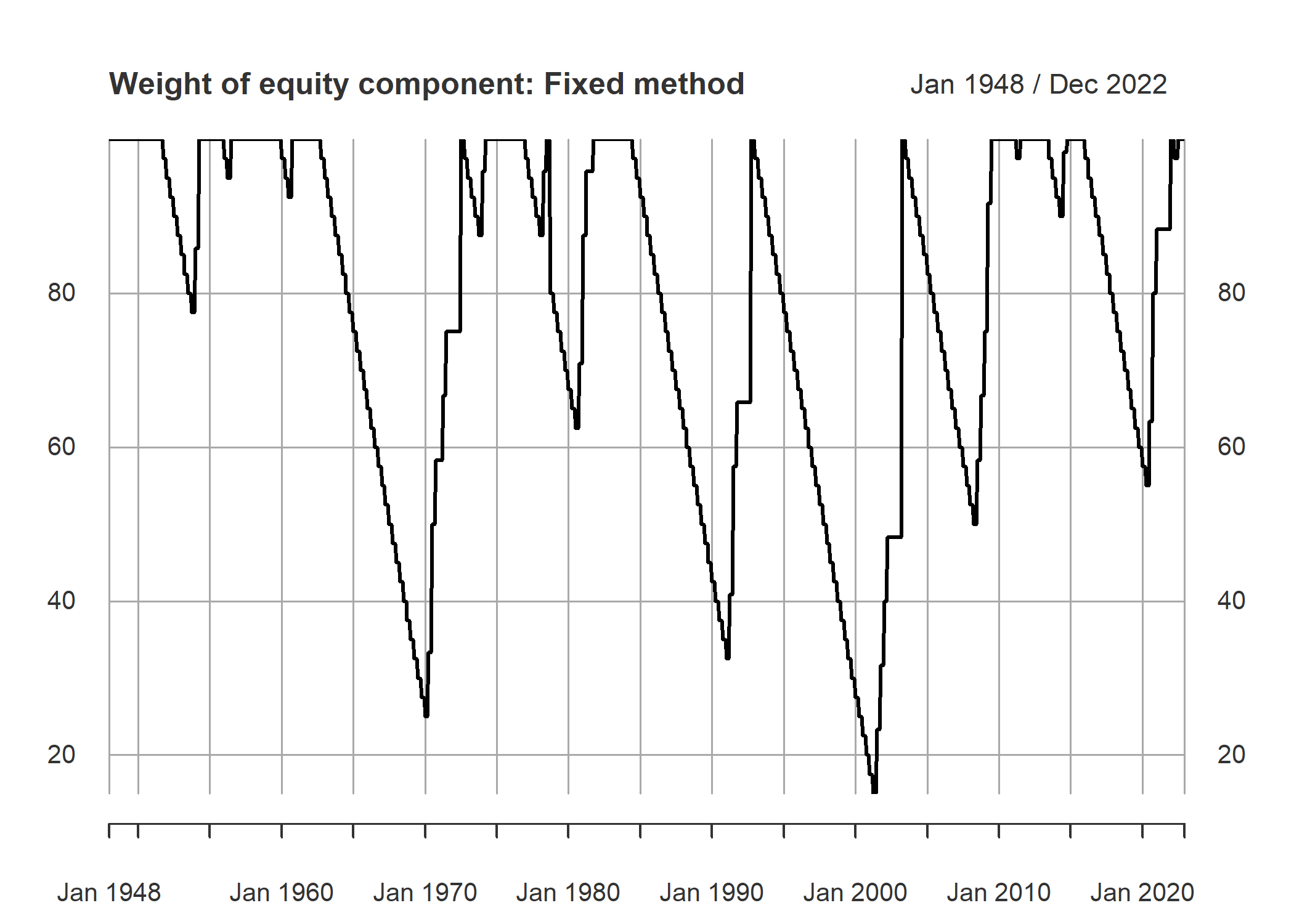
For getting the weights, I used a definition of recessions. That is 2 consequential negative real seasonal growth. begging from a full equity portfolio, each period we reduce equity weigh. And when a recession happens, we buy as much as we can. For the timing and amounts of change per period, I used following two:
- If the sign of real GDP growth negatives for 2 consecutive time, we increase equity share by 50/3 percent per season. If it is 0, 1 or -1, we increase it by half of this amount, 50/6 percent. When real GDP growth has positive signs, a couple of predefined series been will be considered. One is a sequence series from 100 to zero that reduced 2.5 percent per month and stays at zero after reaching to that amount.
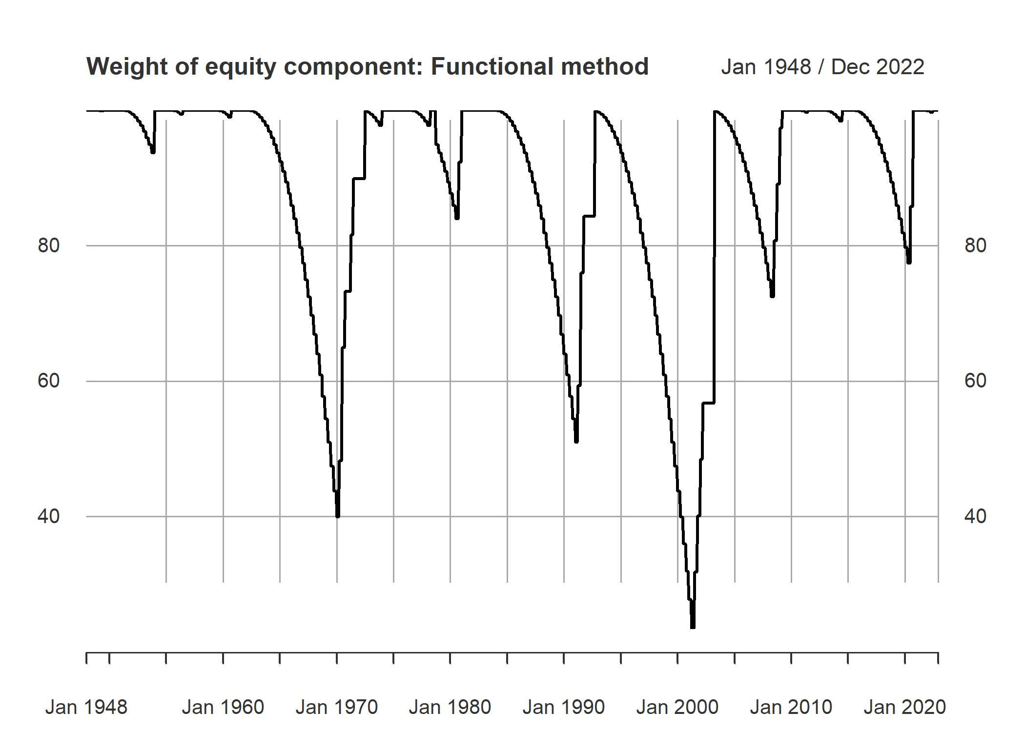
- A second series is made by following function at 1-unit intervals
from 1 to 40:
Where i denote time elapsed from latest 2 consecutive negative sign. This function implies that the amount of cash will increase as time passes and after 40 season or 10 years, the portfolio only consists of cash. We take 3 season as resting period after a 2 negative sign reset occurrence. That is 3 season after series of good economic growth data happened, the weight of equities, W_eq, in the portfolio will begin to decrease.
A final matter is that third announcement of real GDP growth by Bureau of Economic Analysis is announced almost 3 months after end of season. We take this revised number and date, as the basis for the periods. In other words, since the information about real GDP growth is available with a season lag, the series are calculated by a season lag too. A visual chart for the two series from 1948 are as follows.
# Functions resulting weight of equity in the portfolio

GDP.trigger<- function( x =  gGDPreal, treshold = 0,
                        n.negative = 2,
                        functional.change = TRUE, n.rebalance.pos = 3,
                        n.rebalance.neg = 3,
                        T.addition= 3,
                        v.change.pos = -10, v.change.neg = 50){
  sign_x<-  sign (x - treshold)
  trigger_x<- lag( sign_x, 1) + lag( sign_x, 0)
  trigger_x<- trigger_x[ -1,]
  weight_eq<- NULL
  rec.ind<- 0
  w.e<- 100
  change.pos.fun<- NULL
  for(j in 1 : 40){
    temp<- ( 1- (1-( j/40)^2))
    temp<- 1 - temp
    change.pos.fun<- c( change.pos.fun, temp)
  }
  change.pos.fun<- change.pos.fun*100
  change.pos.fix<- seq( from = 100 , 0, by = v.change.pos/4)
  change.pos.fix[is.na(change.pos.fix)]<-0
  #change.pos.fun<- c( rep( 100, 12), change.pos.fun)
  for ( i in 1 : length( trigger_x)){
    trigger<- trigger_x[i]

    if( trigger <= 0)  rec.ind<- i
    elapsed<- i - rec.ind


    if( functional.change == FALSE){
      if( trigger <= -2 ) w.e<- min( w.e + v.change.neg/n.rebalance.neg , 100)
      if( trigger > -2 & trigger < 2) w.e<- min( w.e + v.change.neg/(n.rebalance.neg*2) , 100)
      if( elapsed > T.addition){
        if( trigger >= 2) w.e<- max( change.pos.fix[elapsed - T.addition] , 0)
      }
    }
    if( functional.change == TRUE){
      #list.change.pos<- change.pos.fun[ c( rep(FALSE, 11), TRUE ) ]

      if( trigger<= -2 ) w.e<- min( w.e + v.change.neg/n.rebalance.neg , 100)
      if( trigger> -2 & trigger< 2) w.e<- min( w.e + v.change.neg/(n.rebalance.neg*2) , 100)
      if( elapsed > T.addition){
        if( trigger>= 2) w.e<- max( change.pos.fun[elapsed - T.addition] , 0)
      }
    }
    weight_eq<- c( weight_eq, w.e)

  }
  return(weight_eq)
}

s_GDP_trig<- GDP.trigger(x =  gGDPreal, treshold = 0,
                         n.negative = 2,
                         functional.change = FALSE, n.rebalance.pos = 3,
                         n.rebalance.neg = 3,
                         T.addition= 3,
                         v.change.pos = -10, v.change.neg = 50)

# making index monthly instead of seasonally
m_GDP_trig<- rep(s_GDP_trig, each =3)
gdp_date<- index(gGDPreal)
gdp_date<- c( gdp_date, gdp_date[ length(gdp_date)]+30)
gdp_date<- c( gdp_date, gdp_date[ length(gdp_date)]+31)


# Changing index to release date of data
releasedate<- gdp_date %m+% months(6)
gdp_indx<- as.yearmon(seq( from = releasedate[2],
                           to = releasedate[ length(releasedate)], by = 'm'))
m_GDP_trig<- as.xts( as.numeric(m_GDP_trig), order.by = gdp_indx)

# plotting the weights
plot(m_GDP_trig, main = "Weight of equity component: Fixed method")
# getting equity weights by function method
s_GDP_trig_fun<- GDP.trigger(x =  gGDPreal, treshold = 0,
                         n.negative = 2,
                         functional.change = TRUE, n.rebalance.pos = 3,
                         n.rebalance.neg = 3,
                         T.addition= 3,
                         v.change.pos = -10, v.change.neg = 50)
m_GDP_trig_fun<- rep(s_GDP_trig_fun, each =3)
m_GDP_trig_fun<- as.xts( as.numeric(m_GDP_trig_fun), order.by = gdp_indx)
# plotting the weights
plot(m_GDP_trig_fun, main = "Weight of equity component: Functional method")
#
#
Backtesting
Creating 500 random portfolios that each had 30 assets in them. Value weighted portfolio is based on market equity of constituent assets, that is, number of outstanding shares time end of month price of a share. Equal weighted portfolio gives equal weights to each asset. These weights are rebalanced at each period. For returns, monthly returns reported by CCM is used (I did not go into the details but these reported returns are significantly different from EOM price growths). For return on cash, 4 weekly treasury bill yields were used.
# function calculating returns of the portfolio

ret_portfo<- function( Begin_syms. = Begin_syms, data = data,
                       tradables_ones = tradables_ones,
                       sym_ind_maker = sym_ind_maker.,
                       N_sym_portfolio = N_sym_portfolio,
                       use.reported.ret = TRUE){

  ## stage 1, choosing the symbols in porfolio in each date
  ## the function is bacwark looking
  N_Dobservation<- last( tradables_ones$datadate)
  sym_set <- rbind(Begin_syms.)
  sym_port <- NULL
  change_sym_length<- 1
  while (change_sym_length > 0) {
    excluded_ones <- NULL
    n_date_row<- dim( sym_set)[1]
    for (i in 1 : ncol( sym_set)) {
      sym_current<- sym_set[ dim( sym_set)[1] , i]
      data_sym <- subset(data, data$GVKEY == sym_current &
                           data$datadate > tradables_ones$datadate[n_date_row])
      change_eligible <- c( 0 , diff(data_sym$eligible))
      nlastdate_sym <- last( data_sym$datadate)
      temp <- NULL
      if( nrow(data_sym) == 0){
        temp <- cbind.data.frame(
          sym = sym_current,
          date = tradables_ones$datadate[n_date_row+1],
          eligible = 0,
          i = i
        )
        excluded_ones <- rbind.data.frame(excluded_ones, temp)
      } else {
      if (length(unique (change_eligible)) > 1 | nlastdate_sym < N_Dobservation) {
        chaange_ind <- first(which(change_eligible != 0))
        if( length(chaange_ind) > 0 ){
        temp <- cbind.data.frame(
          sym = sym_current,
          date = data_sym$datadate[chaange_ind],
          eligible = data_sym$eligible[chaange_ind],
          i = i
        )
        excluded_ones <- rbind.data.frame(excluded_ones, temp)
        } else {
          if( nlastdate_sym < N_Dobservation ){
            temp <- cbind.data.frame(
              sym = sym_current,
              date = last( data_sym$datadate),
              eligible = last( data_sym$eligible),
              i = i
            )
          }
        }
        excluded_ones <- rbind.data.frame(excluded_ones, temp)
      }
      }
    }

    change_sym_length <- length(excluded_ones)
    if (change_sym_length > 0) {
      change_date <- min(excluded_ones$date)
      excld_syms <-
        subset(excluded_ones, excluded_ones$date == change_date)
      change_syms <- unique(excld_syms$sym)

      n_sym_exclude <- length(change_syms)
      lag_syms<- sym_set [ dim(sym_set)[1],]
      remained_syms <- lag_syms[ -which( lag_syms %in% change_syms)]
      available_syms <-
        tradables_ones[ which(tradables_ones$datadate ==
                               change_date), ]
      available_syms<- available_syms[ -1]
      available_syms <-  as.integer( available_syms[ !is.na( available_syms)])
      available_syms <-
        available_syms[ -which( available_syms %in% remained_syms)]
      added_syms <- sample(available_syms, n_sym_exclude)
      new_syms <- c(remained_syms, added_syms)
      ##
      ## change dim
      n.row <- which(tradables_ones$datadate == change_date)
      n.row<- n.row - nrow(sym_set) -1
      if( n.row > 0){
      temp1 <- matrix( rep(sym_set[dim(sym_set)[1],],  n.row),
                       nrow = n.row, byrow = TRUE)
      sym_set <- rbind(sym_set, temp1)
      rm(temp1)
      }
      sym_set <- rbind(sym_set, new_syms)
      excluded_ones<- NULL
    } else {
      n.row <- dim( tradables_ones)[1]
      n.row<- n.row - nrow(sym_set)
      temp2 <- matrix( rep(sym_set[dim(sym_set)[1],], times = n.row),
                       nrow = n.row, byrow = TRUE)
      sym_set <- rbind(sym_set, temp2)
      rm(temp2)
      excluded_ones<- NULL
    }
  }


  sym_set<- as.data.frame(sym_set)
  sym_set$date<- tradables_ones$datadate

  # subset data for portfolio
  port_sym_universe<- unique(unlist(sym_set[ , - dim(sym_set)[2]]))
  port_data<- subset( data, data$GVKEY %in% port_sym_universe)
  port_data<- subset( port_data,
                      port_data$datadate >= (as.Date(begin_date) -365))
  # making Price matrix as data.frame
  Prices_sym<- as.xts( rep(0 , length(sym_set$date)),
                   order.by = sym_set$date, dateFormat="Date")
  for ( i in 1 : length ( port_sym_universe)){
    temp0<- subset( port_data, port_data$GVKEY == port_sym_universe[ i])
    temp1<- temp0$prccm
    temp1<- as.xts( temp1, order.by = temp0$datadate, dateFormat="Date" )
    Prices_sym<- merge( Prices_sym, temp1)
  }
  Prices_sym<- Prices_sym[ , -1]
  colnames(Prices_sym)<- port_sym_universe
  # log return
  ret_syms<- diff( log( Prices_sym))
  ret_syms<- ret_syms[ -1,]
  ret_syms<- ret_syms[ sym_set$date]
  #Prices_sym["2000-05-31::2000-07-31"]
  # ME matrix
  ME_sym<- as.xts( rep(0 , length(sym_set$date)),
                   order.by = sym_set$date)
  for ( i in 1 : length ( port_sym_universe)){
    temp0<- subset( port_data, port_data$GVKEY == port_sym_universe[ i])
    temp1<- temp0$ME
    temp1<- as.xts( temp1, order.by = temp0$datadate )
    ME_sym<- cbind.xts( ME_sym, temp1)
  }
  ME_sym<- ME_sym[ , -1]
  colnames(ME_sym)<- port_sym_universe
  ME_sym<- lag.xts(ME_sym)
  ME_sym<- ME_sym[ -1,]
  ME_sym<- ME_sym[ sym_set$date]
  #length(temp)<- length(sym_set$date)
  #monthly return as reported in the dataset
  #trt1m
  Trm_sym<- as.xts( rep(0 , length(sym_set$date)),
                   order.by = sym_set$date)
  for ( i in 1 : length ( port_sym_universe)){
    temp0<- subset( port_data, port_data$GVKEY == port_sym_universe[ i])
    temp1<- temp0$trt1m
    temp1<- as.xts( temp1, order.by = temp0$datadate )
    Trm_sym<- cbind.xts( Trm_sym, temp1)
  }
  Trm_sym<- Trm_sym[ , -1]
  Trm_sym<- Trm_sym/100
  colnames(Trm_sym)<- port_sym_universe
  Trm_sym<- Trm_sym[ sym_set$date]

  ### Chosing type of return
  if( use.reported.ret == TRUE){
    ret_syms<- Trm_sym
  }
  #colMeans(Trm_sym, na.rm = TRUE) - colMeans(ret_syms, na.rm = TRUE)

  # indicating subsets of symbols for each period
  sym_port_indc<- NULL
  for( j in 1 : nrow(sym_set)){
    temp<- sym_ind_maker( sym_set. = sym_set[ j,],
                          sym_universe = port_sym_universe)
    sym_port_indc<- rbind(sym_port_indc, temp)
  }

  # sum(sym_port_indc[1,] %in% port_sym_universe )
  # sum(sym_port_indc)/20
  colnames(sym_port_indc)<- port_sym_universe
  sym_port_indc<- as.data.frame(sym_port_indc)
  sym_port_indc<- as.xts( sym_port_indc, order.by =  sym_set$date)
  #### Weight Matrix
  equal_replica<- rep( 1/ N_sym_portfolio , length(port_sym_universe))
  weight_portf_sym<- sym_port_indc %*% diag(equal_replica)
  #weight_portf_sym<- weight_portf_sym[ -1,]

  # Market equity weigthed
  ME_port<- NULL
  for(i in 1 : nrow(sym_set)){
    temp<- NULL
    index_sym_incl<- as.logical(sym_port_indc[i,])
    ME_sym<- na.locf(ME_sym)
    temp<- ME_sym[ i, index_sym_incl]
    #if(sum(is.na(temp))>0){
    #  temp[is.na(temp)]<- mean(temp, na.rm = TRUE)
    #}
    ME_port<- rbind(ME_port, temp)
  }

  sum_ME<-  rowSums(ME_port, na.rm = TRUE)
  W_port_ME<- ME_port/sum_ME

  ## equity components return
  #ret_syms_date<- ret_syms[ index( ME_port),]
  ret_syms_date<- ret_syms
  ret_sym_port<- NULL
  for(i in 1 : nrow(sym_set)){
    temp<- NULL
    index_sym_incl<- as.logical(sym_port_indc[i,])
    temp<- ret_syms_date[ i, index_sym_incl]
    ret_sym_port<- rbind(ret_sym_port, temp)
  }

  # Rebalanced equal weight

  # Rebalanced fixed weight at start
  ret_sym_port0<- ret_sym_port
  ret_sym_port0[is.na(ret_sym_port)] <- 0
  ret_port_wME<- diag(ret_sym_port0 %*% t(W_port_ME))
  ret_port_wME<- as.xts( ret_port_wME, order.by = index( ret_sym_port0))
  # Rebalanced annually

  # Rebalanced by triger

  # portfolio returns
  ret_syms0 <-  ret_syms
  ret_syms0[is.na(ret_syms)] <- 0
  port_return_eq<- diag(   ret_syms0 %*% t(weight_portf_sym))
  port_return_eq<- as.xts( port_return_eq, order.by = index( ret_syms))

  # testing function
  #ret_check<- rowSums(ret_sym_port0)/20

  # returns 1st equal weight, second value weight
  port_ret<- cbind(port_return_eq, ret_port_wME)

  return(port_ret)
}

# creating fist observation randomly by predefined seed
Begin_syms_m <- NULL
for( i in 1 : n.sim){
  set.seed(seed_value+i-1)
  temp<- NULL
  temp<- sample(begin_eligible, N_sym_portfolio )
  Begin_syms_m<- rbind(Begin_syms_m, temp)
}


return_portfo<- ret_portfo( Begin_syms. = Begin_syms, data = data,
                       tradables_ones = tradables_ones, N_sym_portfolio = 50)
#322 407 484
# the code give error for 322, 407, 484 beginning sets
# it should be checked, for now they are excluded
simulation_set<- 1:500
simulation_set<- simulation_set[ !c(simulation_set %in% c(322, 407, 484 ))]

# getting results of simulation: to be a faster code later
ret_matrix<- NULL
for(i in 1 : nrow(simulation_set)){
  temp<- ret_portfo( Begin_syms. = Begin_syms, data = data,
                     tradables_ones = tradables_ones, N_sym_portfolio = 50,
                     use.reported.ret = TRUE)
  ret_matrix<- cbind(ret_matrix, temp)
}

# saving simulation results
#save(ret_matrix, file = "ret_30_500.R")
# plot(cumprod( 1+ ret_matrix[,1]))

library(zoo)
library(xts)

load("ret_30_500.R")
load("gen_data.Rdata")


# return_portfolio

index(ret_matrix) <- as.yearmon(index(ret_matrix))

# returns of equal weighted portfolios
Eq_W_portfolio<- NULL
for(i in 1:(ncol(ret_matrix)/2)) Eq_W_portfolio<- cbind(Eq_W_portfolio, ret_matrix[, (2*i-1)])

# returns of value weighted portfolios
Va_W_portfolio<- NULL
for(i in 1:(ncol(ret_matrix)/2)) Va_W_portfolio<- cbind(Va_W_portfolio, ret_matrix[, (2*i)])

# simple method
# vector of equity weight
W_vec<- m_GDP_trig[ index(Eq_W_portfolio)]/100
# matrix of equity weight
W_matrix<- matrix(W_vec, nrow= nrow(W_vec),
                  ncol=ncol(Eq_W_portfolio), byrow=FALSE)
# tbill return time weight
ret_TB_vec<- TB1MS * ( 1 - W_vec)
ret_TB_matrix<- matrix(ret_TB_vec, nrow= nrow(ret_TB_vec),
                       ncol=ncol(Eq_W_portfolio), byrow=FALSE)
# portfolio returns for equal weight and value weight
ret_tot_eqW<- Eq_W_portfolio *W_matrix + ret_TB_matrix
ret_tot_valW<- Va_W_portfolio *W_matrix + ret_TB_matrix
####################
# Function method
# vector of equity weight
W_vec_fun<- m_GDP_trig_fun[ index(Eq_W_portfolio)]/100
# matrix of equity weight
W_matrix_fun<- matrix(W_vec_fun, nrow= nrow(W_vec_fun),
                  ncol=ncol(Eq_W_portfolio), byrow=FALSE)
# tbill return time weight
ret_TB_vec_fun<- TB1MS * ( 1 - W_vec_fun)
ret_TB_matrix_fun<- matrix(ret_TB_vec_fun, nrow= nrow(ret_TB_vec_fun),
                       ncol=ncol(Eq_W_portfolio), byrow=FALSE)
# portfolio returns for equal weight and value weight
ret_tot_eqW_fun<- Eq_W_portfolio *W_matrix_fun + ret_TB_matrix_fun
ret_tot_valW_fun<- Va_W_portfolio *W_matrix_fun + ret_TB_matrix_fun


port_names<- c( "Eq_W_portfolio", "ret_tot_eqW", "ret_tot_eqW_fun",
                "Va_W_portfolio", "ret_tot_valW", "ret_tot_eqW_fun" )

#save(Eq_W_portfolio, ret_tot_eqW, ret_tot_eqW_fun,                 Va_W_portfolio, ret_tot_valW, ret_tot_eqW_fun, file = "ret_port_all_data.Rdata")
Table 1 shows performance metrics for equal weighted portfolio and derived portfolios from it by changing the interest-bearing cash in the portfolio. Derived portfolios beta with respect to S&P500 index is less than original random portfolios. Annualized return shows a slight improvement. Yet the overall change is related to variance of the return series. Sharp and Information ratio improve substantially. The fixed method of increasing cash weight by 10 percent per year overwhelms the functional method.
| Value Weighted mean | vl sd | transformed vl mean | tr vl sd | fun transformed vl mean | fun vlsd | |
|---|---|---|---|---|---|---|
| Beta | 0.8318 | 0.0694 | 0.6098 | 0.04847 | 0.3195 | 0.01466 |
| Annualized returns: Arthemetic | 0.122 | 0.01026 | 0.1094 | 0.007691 | 0.06021 | 0.001949 |
| Annualized returns: Geometric | 0.1107 | 0.01134 | 0.1043 | 0.008256 | 0.05969 | 0.002044 |
| mean sd returns | 0.1817 | 0.01176 | 0.1404 | 0.0102 | 0.06487 | 0.002299 |
| Max DrawDown | 0.5387 | 0.07406 | 0.4461 | 0.0396 | 0.2221 | 0.01873 |
| Sharp ratio: Arthemetic | 0.6122 | 0.076 | 0.746 | 0.07393 | 0.9213 | 0.04459 |
| Sharp ratio: Geometric | 0.6122 | 0.076 | 0.746 | 0.07393 | 0.9213 | 0.04459 |
| Upside Potential Ratio | 0.7958 | 0.03691 | 0.8264 | 0.0392 | 0.8334 | 0.02962 |
| Information Ratio | 0.2689 | 0.07675 | 0.265 | 0.06509 | -0.1092 | 0.02034 |
Table 1 Performance Measures Equal Weighted
| Value Weighted mean | vl sd | transformed vl mean | tr vl sd | fun transformed vl mean | fun vlsd | |
|---|---|---|---|---|---|---|
| Beta | 0.8318 | 0.0694 | 0.6098 | 0.04847 | 0.3195 | 0.01466 |
| Annualized returns: Arthemetic | 0.122 | 0.01026 | 0.1094 | 0.007691 | 0.06021 | 0.001949 |
| Annualized returns: Geometric | 0.1107 | 0.01134 | 0.1043 | 0.008256 | 0.05969 | 0.002044 |
| mean sd returns | 0.1817 | 0.01176 | 0.1404 | 0.0102 | 0.06487 | 0.002299 |
| Max DrawDown | 0.5387 | 0.07406 | 0.4461 | 0.0396 | 0.2221 | 0.01873 |
| Sharp ratio: Arthemetic | 0.6122 | 0.076 | 0.746 | 0.07393 | 0.9213 | 0.04459 |
| Sharp ratio: Geometric | 0.6122 | 0.076 | 0.746 | 0.07393 | 0.9213 | 0.04459 |
| Upside Potential Ratio | 0.7958 | 0.03691 | 0.8264 | 0.0392 | 0.8334 | 0.02962 |
| Information Ratio | 0.2689 | 0.07675 | 0.265 | 0.06509 | -0.1092 | 0.02034 |
Table 2 Performance Measures Value Weighted
| Mkt.RF | R2 Mkt.RF | SMB | R2 SMB | HML | R2 HML | |
|---|---|---|---|---|---|---|
| Eq Weight mean | 0.004096 | 0.7796 | 0.002021 | 0.08454 | 1.845e-05 | -0.0005217 |
| eq sd | 0.0001699 | 0.02183 | 0.0002209 | 0.01571 | 0.0002305 | 0.001503 |
| transformed eq mean | 0.003068 | 0.708 | 0.001707 | 0.09741 | 6.322e-05 | -0.0008323 |
| tr sd | 0.0001156 | 0.01666 | 0.0001311 | 0.01106 | 0.0001418 | 0.001144 |
| fun transformed eq mean | 0.003564 | 0.7494 | 0.001919 | 0.09662 | 6.86e-05 | -0.0007547 |
| fun sd | 0.0001359 | 0.01792 | 0.0001564 | 0.01209 | 0.0001702 | 0.001248 |
| Value Weighted mean | 0.009649 | 0.7014 | 0.002849 | 0.02852 | -0.001752 | 0.01354 |
| vl sd | 0.0006837 | 0.05102 | 0.001004 | 0.01869 | 0.001212 | 0.0146 |
| transformed vl mean | 0.007129 | 0.6423 | 0.002399 | 0.03247 | -0.001012 | 0.007649 |
| tr vl sd | 0.0004536 | 0.05256 | 0.000569 | 0.01392 | 0.0007552 | 0.008965 |
| fun transformed vl mean | 0.003564 | 0.7494 | 0.001919 | 0.09662 | 6.86e-05 | -0.0007547 |
| fun vlsd | 0.0001359 | 0.01792 | 0.0001564 | 0.01209 | 0.0001702 | 0.001248 |
Tabel 3 OLS on FF3 individually
| Mkt.RF | SMB | HML | R2 | |
|---|---|---|---|---|
| Eq Weight mean | 0.004228 | 0.0005516 | 0.001545 | 0.83 |
| eq sd | 0.0001672 | 0.0001937 | 0.0002412 | 0.01934 |
| transformed eq mean | 0.003139 | 0.0006302 | 0.001233 | 0.7636 |
| tr sd | 0.0001203 | 0.0001168 | 0.0001683 | 0.01731 |
| fun transformed eq mean | 0.003658 | 0.0006618 | 0.00142 | 0.8059 |
| fun sd | 0.0001409 | 0.0001387 | 0.000198 | 0.01793 |
| Value Weighted mean | 0.01006 | -0.001008 | 0.001493 | 0.7192 |
| vl sd | 0.0006692 | 0.0008933 | 0.001258 | 0.04699 |
| transformed vl mean | 0.007419 | -0.0003891 | 0.00144 | 0.6581 |
| tr vl sd | 0.000476 | 0.0005218 | 0.0008624 | 0.0508 |
| fun transformed vl mean | 0.003658 | 0.0006618 | 0.00142 | 0.8059 |
| fun vlsd | 0.0001409 | 0.0001387 | 0.000198 | 0.01793 |
Table 2 illustrates performance metrics for value weighted portfolio and related derived portfolios by changing the weights of interest-bearing cash in the portfolio. Except for the sharp ratio, the functional derivation is almost worst in every case. For fixed method, the Beta with the index is less than the beta of the original series. Annualized return shows a half percent reduction. As with equal weighted case, the overall change is stemmed by the change in the variance of the return series. Sharp ratios increase but Information ratio shows no improvement.
Averaged results of regression on Fama French 3 factors (table 3) shows that these factors explain the variations in the return series very well. Adjusted R squares are high, ranging from 0.83 to 0.66. Future the numbers shows little variations across the 500 created portfolios.
Table 4 shows the coefficients of Fama French 3 Factors when they are sole regressor with a constant. HML factor has no significant contribution in explaining these variations. Overall excess return of the market portfolio seems to be a very good and powerful explanatory variable.
Conclusion
Empirical results on cash and equal weight equity rebalanced portfolios showed improvements over almost all considered performance metrics. This result shows that variable amount of cash based on last negative real GDP growth can result in less risky portfolio while the returns are the same.
For value weighted portfolio, the results were not as satisfactory. In addition, considering survivorship bias due to delisting and delisting returns and affect performance on both portfolios. Also, one can consider the same method of making portfolios but without rebalancing (buy and hold method).
For further work, one can investigate negative beta of the returns with excess return of the market portfolio over time and economic cycles, and similarities and dissmilarities to 40/60 portfolio.
Looking from another viewpoint, maybe Schumpeter creative destruction is source of value in more than one way :) But this statement needs more rigorous work than what I wrote. Anyhow the results were pretty surprising for me, And I loved them :D