Price limit and Markov Chains
One of the things that bothers me about Tehran Stocks Market is price limit. It simply distorts market adjustment procedure and causes binomial changes in liquidity. Since it exist and my retirement portfolio was subject to it several times, I saw a need for taking a look at it. Another thing that is tightly related to this is that final price is weighted average of intraday trades. As a result it is possible that a positive shock happens and since the effect is perceived by all participants to be more than the limit, the price would not change and liquidity becomes zero. Although an extreme case, yet this extremities give insight about what need to be examined.
I like to see this changes of regimes as Markov chains. Ever since a professor of mine mentioned that human civilization could follow a Markov chain, I am somehow obsessed with Markov chains. In this post I would look whether this obsession has anything useful about it :)
For the distribution of returns, censored normal distribution seems logical so I proceed with that.
From 28-06-2010 to 23-05-2015 the price limit was symmetric and was 4 percent of the asset prices. Since 23-05-2015 the limit was ameliorated and changed to 5 percent of asset prices. I first take a glimpse on first period and then I take a better look at current period.
High of the day matters
Since the close price is the weighted average of trades, for knowing whether the process has changed regimes we need to used the information that exist in high or low of the day. Maybe some time ago I would have never imagined that high of the day has any such important information in it, yet after looking more closely, I saw that if the high or low is equal to last traded price (in my data it is called LCLOSE) and both equal to extremes of price limit, these could contain some information about regime changes.
vars<-c("FIRST", "HIGH", "LOW", "CLOSE",
        "LPRICE","LCLOSE")

WDATA[,paste0("ln",vars)] <- apply(WDATA[,c("FIRST", "HIGH", "LOW", "CLOSE",
                                            "LPRICE", "LCLOSE" )],2,log)
WDATA[is.nan.data.frame(WDATA)] <- 0

WDATA[,13:18]<- apply(WDATA[,13:18],2,function(x) { x[ x == -Inf ] = 0 ; x })

#returns

WDATA$r.H.LC<- WDATA$lnLCLOSE -  WDATA$lnLPRICE
WDATA$retCL<-WDATA$lnCLOSE -  WDATA$lnLPRICE

WDATA$max4p<- floor(WDATA$LPRICE * 1.04)
WDATA$min4p<- ceiling(WDATA$LPRICE * .96)
WDATA$max5p<- floor(WDATA$LPRICE * 1.05)
WDATA$min5p<- ceiling(WDATA$LPRICE * .95)

WDATA.4p<- subset( WDATA, WDATA$DATE >= as.Date("2010-06-27") & WDATA$DATE < as.Date("2015-05-23"))

WDATA.4p$r.H.LC[ WDATA.4p$r.H.LC > .04]<- .04
WDATA.4p$r.H.LC[ WDATA.4p$r.H.LC < -.04]<- -.04

WDATA.4p$ind4p<- 0
WDATA.4p$ind4p[WDATA.4p$max4p <= WDATA.4p$LCLOSE] <- 1
WDATA.4p$ind4p[WDATA.4p$r.H.LC == .04] <- 1

WDATA.4p$ind_4p<- 0
WDATA.4p$ind_4p[WDATA.4p$min4p >= WDATA.4p$LOW] <- -1
WDATA.4p$ind_4p[WDATA.4p$r.H.LC == -.04] <- -1

WDATA.4p$Lind4p<- c(NA, WDATA.4p$ind4p[- length(WDATA.4p$ind4p)])
Lets see how the sequences of staying at limit would last:
path = "C:/Users/msdeb/Documents/Stock and trades/"
setwd(path)
load(".Rdata")
library(pander)
t<- rle(WDATA.4p$ind4p)
L1<- t$lengths[t$values == 1]
pander(summary(as.factor(L1)))
| 1 | 2 | 3 | 4 | 5 | 6 | 7 | 8 | 9 | 10 | 11 | 12 | 13 | 14 | 15 | 16 | 17 |
|---|---|---|---|---|---|---|---|---|---|---|---|---|---|---|---|---|
| 17809 | 5907 | 2258 | 1076 | 571 | 324 | 160 | 97 | 59 | 43 | 31 | 25 | 13 | 7 | 11 | 9 | 6 |
| 18 | 19 | 20 | 21 | 22 | 24 | 26 | 36 | 38 |
|---|---|---|---|---|---|---|---|---|
| 4 | 1 | 4 | 1 | 1 | 1 | 1 | 1 | 1 |
t_ <- rle(WDATA.4p$ind_4p)
L_1<- t_$lengths[t_$values == -1]
pander(summary(as.factor(L_1)))
| 1 | 2 | 3 | 4 | 5 | 6 | 7 | 8 | 9 | 10 | 11 | 12 | 13 | 14 | 15 | 16 |
|---|---|---|---|---|---|---|---|---|---|---|---|---|---|---|---|
| 23860 | 9707 | 4077 | 2025 | 1197 | 678 | 404 | 311 | 198 | 133 | 89 | 72 | 46 | 39 | 24 | 24 |
| 17 | 18 | 19 | 20 | 21 | 22 | 23 | 24 | 25 | 26 | 27 | 30 | 42 |
|---|---|---|---|---|---|---|---|---|---|---|---|---|
| 17 | 14 | 12 | 4 | 2 | 6 | 5 | 2 | 1 | 4 | 3 | 1 | 1 |
The length of sequences shows some persistence lets look more thoroughly by fitting a Markov chain:
WDATA.4p$ind.cnsr<- WDATA.4p$ind_4p + WDATA.4p$ind4p

library(markovchain)

MC4p<- markovchainFit(as.character(WDATA.4p$ind.cnsr), method="mle")
# conditional distribution
mcE <- new("markovchain", states = c("-1", "0", "1"),
           transitionMatrix = MC4p$estimate@transitionMatrix)

pander(MC4p$estimate@transitionMatrix)
| -1 | 0 | 1 | |
|---|---|---|---|
| -1 | 0.5055 | 0.4247 | 0.06988 |
| 0 | 0.08733 | 0.8619 | 0.05074 |
| 1 | 0.09883 | 0.4745 | 0.4267 |
assessStationarity(WDATA.4p$ind.cnsr, floor(length(WDATA.4p$ind.cnsr)/5))
## The assessStationarity test statistic is: 77822.36 the Chi-Square d.f. are: 679404 the p-value is: 1
## $statistic
## [1] 77822.36
##
## $p.value
## [1] 1
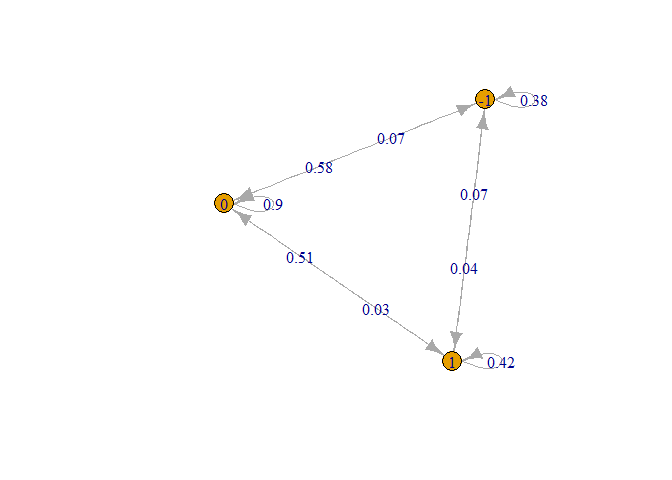
plot(mcE)
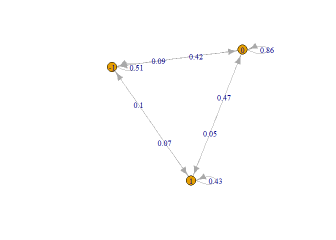
The series are not rejected to be stationary. And we see that there is some probability that the states recurs. An interesting matter is that there are small probabilities that the process changes from maximum limit to minimum limit. If I have had known this, I would have produced more return on my retirement portfolio.
Now that the analyse seems not futile, let me proceed to the current 5 percent price limit period.
WDATA.5p<- subset( WDATA, WDATA$DATE > as.Date("2015-05-23"))
na.omit.WDATA.5p<- WDATA.5p[complete.cases(WDATA.5p$r.H.LC),]
library( ggplot2)
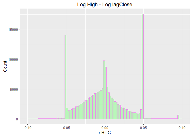
ggplot(data=na.omit.WDATA.5p, aes(na.omit.WDATA.5p$r.H.LC)) +
geom_histogram(breaks=seq(-.1, 0.1, by = 0.002),
col="violet",
fill="green",
alpha = .2) +
labs(title="Log High - Log lagClose") +
labs(x="r.H.LC", y="Count")
ggplot(data=na.omit.WDATA.5p, aes(na.omit.WDATA.5p$retCL)) +
  geom_histogram(breaks=seq(-.1, 0.1, by = 0.002),
                 col="violet",
                 fill="green",
                 alpha = .2) +
  labs(title="Return Based on Close") +
  labs(x="retCL", y="Count")

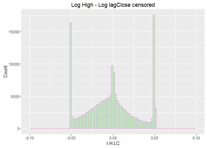
The distribution of returns has values more than 5 percent, since the process is censored, I would make it completely censored by letting those values to be equal to price limit extremes (these values are related to the times that an asset being not tradable become tradable again).
WDATA.5p$r.H.LC[ which( WDATA.5p$r.H.LC > .05)]<- .05
WDATA.5p$r.H.LC[ which( WDATA.5p$r.H.LC < -.05)]<- -.05


WDATA.5p$ind5p<- 0
WDATA.5p$ind5p[ which( WDATA.5p$max5p == WDATA.5p$LCLOSE)] <- 1
WDATA.5p$ind5p[ which( WDATA.5p$r.H.LC == .05)] <- 1

WDATA.5p$ind_5p<- 0
WDATA.5p$ind_5p[ which( WDATA.5p$min5p == WDATA.5p$LOW)] <- -1
WDATA.5p$ind_5p[ which( WDATA.5p$r.H.LC == -.05)] <- -1

na.omit.WDATA.5p<- WDATA.5p[complete.cases(WDATA.5p$r.H.LC),]

ggplot(data=na.omit.WDATA.5p, aes(na.omit.WDATA.5p$r.H.LC)) +
  geom_histogram(breaks=seq(-.1, 0.1, by = 0.002),
                 col="violet",
                 fill="green",
                 alpha = .2) +
  labs(title="Log High - Log lagClose censored") +
  labs(x="r.H.LC", y="Count")
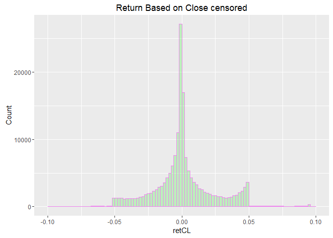
ggplot(data=na.omit.WDATA.5p, aes(na.omit.WDATA.5p$retCL)) +
  geom_histogram(breaks=seq(-.1, 0.1, by = 0.002),
                 col="violet",
                 fill="green",
                 alpha = .2) +
  labs(title="Return Based on Close censored") +
  labs(x="retCL", y="Count")
WDATA.5p$Lind5p<- c(NA, WDATA.5p$ind5p[- length(WDATA.5p$ind5p)])
WDATA.5p$Lind_5p<- c(NA, WDATA.5p$ind_5p[- length(WDATA.5p$ind_5p)])


t<- rle(WDATA.5p$ind5p)
L1<- t$lengths[t$values == 1]
pander(summary(as.factor(L1)))
| 1 | 2 | 3 | 4 | 5 | 6 | 7 | 8 | 9 | 10 | 11 | 12 | 13 | 14 | 15 | 16 | 17 |
|---|---|---|---|---|---|---|---|---|---|---|---|---|---|---|---|---|
| 4700 | 1239 | 499 | 210 | 83 | 70 | 37 | 23 | 20 | 7 | 7 | 9 | 6 | 5 | 5 | 4 | 2 |
| 18 | 19 | 20 | 22 | 24 | 26 | 28 | 31 | 35 | 40 | 53 |
|---|---|---|---|---|---|---|---|---|---|---|
| 3 | 1 | 2 | 2 | 1 | 1 | 1 | 1 | 3 | 1 | 1 |
t_<- rle(WDATA.5p$ind_5p)
L_1<- t_$lengths[t_$values == -1]
pander(summary(as.factor(L_1)))
| 1 | 2 | 3 | 4 | 5 | 6 | 7 | 8 | 9 | 10 | 11 | 12 | 13 | 14 | 15 | 16 | 17 |
|---|---|---|---|---|---|---|---|---|---|---|---|---|---|---|---|---|
| 9745 | 2652 | 913 | 430 | 149 | 94 | 47 | 40 | 31 | 21 | 15 | 11 | 5 | 5 | 10 | 4 | 1 |
| 21 | 22 | 23 | 26 | 28 | 30 |
|---|---|---|---|---|---|
| 1 | 6 | 2 | 1 | 3 | 2 |
Length of being at the extremes sequence seems to behave like previous sequences. So I proceed with the Markov chain estimation.
WDATA.5p$ind.cnsr<- WDATA.5p$ind_5p + WDATA.5p$ind5p
MC5p<- markovchainFit(as.character(WDATA.5p$ind.cnsr), method="mle")
mcE <- new("markovchain", states = c("-1", "0", "1"),
           transitionMatrix = MC5p$estimate@transitionMatrix)

steadyStates(mcE)

##              -1         0          1
## [1,] 0.09752502 0.8517057 0.05076925

assessStationarity(WDATA.5p$ind.cnsr,   floor(length(WDATA.5p$ind.cnsr)/5))

## The assessStationarity test statistic is:  22856.07  the Chi-Square d.f. are:  281646  the p-value is:  1

## $statistic
## [1] 22856.07
##
## $p.value
## [1] 1

plot(mcE)
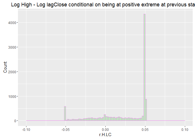
Lets see how the histogram looks like if the previous state was an extreme price state:
na.omit.WDATA.5p<- WDATA.5p[complete.cases(WDATA.5p$r.H.LC),]
na.omit.WDATA.5p<- na.omit.WDATA.5p[ which( na.omit.WDATA.5p$Lind5p == 1) ,]


ggplot(data=na.omit.WDATA.5p, aes(na.omit.WDATA.5p$r.H.LC)) +
  geom_histogram(breaks=seq(-.1, 0.1, by = 0.002),
                 col="violet",
                 fill="green",
                 alpha = .2) +
  labs(title="Log High - Log lagClose conditional on being at positive extreme at previous state") +
  labs(x="r.H.LC", y="Count")
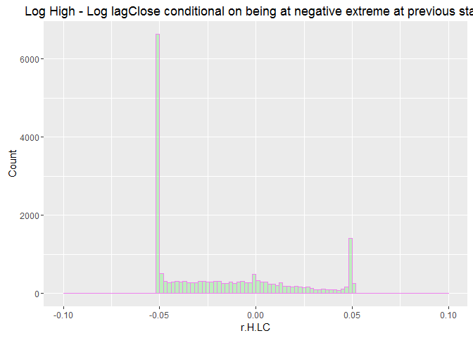
na.omit.WDATA.5p<- WDATA.5p[complete.cases(WDATA.5p$r.H.LC),]
na.omit.WDATA.5p<- na.omit.WDATA.5p[ which( na.omit.WDATA.5p$Lind_5p == -1) ,]


ggplot(data=na.omit.WDATA.5p, aes(na.omit.WDATA.5p$r.H.LC)) +
  geom_histogram(breaks=seq(-.1, 0.1, by = 0.002),
                 col="violet",
                 fill="green",
                 alpha = .2) +
  labs(title="Log High - Log lagClose conditional on being at negative extreme at previous state") +
  labs(x="r.H.LC", y="Count")
Censored Normal Distribution
By following function we could estimate the censored normal distribution parameters:
para = c(0, 1)
ll<-function(para =para , x =WDATA.5p$r.H.LC[!WDATA.5p$Lind5p == 1 ],   censor = .047){
  mu<- para[1]
  sigma<- para[2]
  pnlt<- 0
  if (sigma < 0) {LL<-  10^5}
  else{
  part1<-  pnorm( -censor, mean = mu, sd = sigma, log = TRUE)*(x <= -censor )
  part2<-  dnorm(x, mean = mu, sd = sigma, log = TRUE)*(x > -censor & x < censor )
  part3<-  pnorm(censor, mean = mu, sd = sigma, log = TRUE, lower.tail = FALSE)*(x >= censor )
  LL = -sum( part1 + part2 + part3 + pnlt, na.rm = TRUE)
  }
  return(LL)
}


par.norm<- optim( par = c(0,1), ll,
                  x =WDATA.5p$r.H.LC[( !WDATA.5p$Lind5p == 1) | ( !WDATA.5p$Lind_5p == -1)],
                  censor = .047)$par

par.norm_pc<- optim( par = c(0,1), ll,  x = WDATA.5p$r.H.LC[WDATA.5p$Lind5p == 1 ],   censor = .047)$par

par.norm_nc<- optim( par = c(0,1), ll,  x = WDATA.5p$r.H.LC[WDATA.5p$Lind_5p == -1 ],   censor = .047)$par

pander( par.norm)
-0.002031 and 0.03636
pander( par.norm_pc)
0.04286 and 0.05999
pander( par.norm_nc)
-0.02819 and 0.05349
Return series
Since the liquidity reduces when the price touches its extreme limits, and since the final price is related to the quantity traded, close prices could be different from limits when the process is at the extreme limit states. Let see how the histogram of ratio of return based on close to extreme limits looks like:
deflat<- (WDATA.5p$retCL[which( WDATA.5p$ind5p == 1) ]) /
  (WDATA.5p$r.H.LC[which( WDATA.5p$ind5p == 1) ])
deflat[ deflat > 1]<- 1
deflat[ deflat < 0]<- 0

deflat<- cbind.data.frame(deflat, as.factor("p"))
colnames(deflat)<- c("ratio", "sign")

deflat.n<- ( WDATA.5p$retCL[ which( WDATA.5p$ind_5p == -1) ]) /
  (WDATA.5p$r.H.LC[which( WDATA.5p$ind_5p == -1) ])
deflat.n[ deflat.n > 1]<- 1
deflat.n[ deflat.n < 0]<- 0
deflat.n<- cbind.data.frame( deflat.n, as.factor("n"))
colnames(deflat.n)<- c("ratio", "sign")

deflat<- as.data.frame( rbind( deflat, deflat.n))

deflat[,1]<- as.numeric( deflat[,1])

ggplot( data = deflat, aes(x = ratio , color = sign, fill = sign)) +
  geom_histogram(breaks=seq(-.02, 1, by = 0.02),
                #color=sign, fill = sign,
                #fill=c("green"),
                 alpha = .2) +

  labs(title = "ret Close to ret High Ratio conditional on extreme states") +
  labs(x = "", y = "Count") +
  scale_color_brewer(palette = "Accent") +
  theme_minimal() + theme( legend.position = "top")
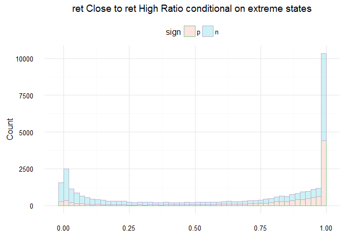
It seems that these are not coming from formal distributions. Computing analytical distribution seems to be not useful for future work so I skip it for now. In case needed I just sample from empirical distribution.
Simulation
Lets simulate and see how the histograms look like:
sim.H.rCl<- function(n = 20000, censor = 0.05, deflat. = deflat, mcE. = mcE){

deflat_p<-deflat.[ deflat.$sign == "p",][,1]
deflat_n<-deflat.[ deflat.$sign == "n",][,1]

x<- rnorm(3*n, mean = par.norm[1], sd = par.norm[2])[200:(3*n)]
x2<- x[ x < censor & x > -censor][1:(n-200)]
x1<- x

mcs<- rmarkovchain(n = n, object = mcE., t0 = "0")[200:n]
x<- rep(NA, length(mcs))
x1<- rep(NA, length(mcs))

x[which(mcs == "1")]<- censor
x[which(mcs == "-1")]<- -censor
x[which(mcs == "0")]<- x2[1: sum( mcs == "0")]

x1[mcs == "1"]<- censor * sample( deflat_p, size = sum(mcs == "1"),  replace = TRUE)
x1[mcs == "-1"]<- -censor  * sample( deflat_n, size = sum(mcs == "-1"),  replace = TRUE)
x1[mcs == "0"]<- x2[1: sum( mcs == "0")]

return(list( sim.r.H.LC = x , sim.retCL = x1))
}

sim <- sim.H.rCl()

sim.r.H.LC <- as.data.frame(sim$sim.r.H.LC)
sim.retCL <- as.data.frame(sim$sim.retCL)
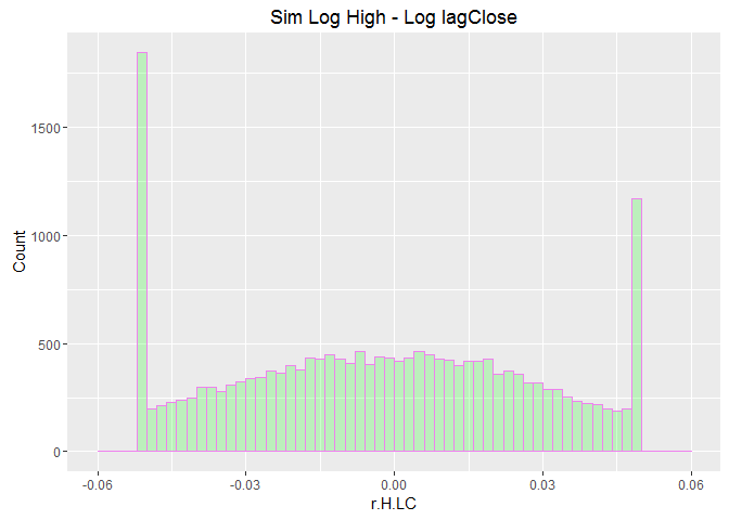
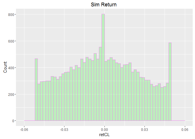
Histograms looks similar to what we saw above yet it put more weigth on negative price limit extreme.
Conclusion
It seemed to me that using Markov chains with censored normal distribution could be helpful and let me to understand the process better. The fact that going from positive limit to negative limit is possible seems to be useful in my future decision making about my retirement portfolio.