Term Structure Of Gold

Minimum-Chi-Square Estimation of Latent Factor Model

In process of fitting wrong models for right reasons, I would try to estimate latent 3 factor model using minimum-chi-square estimation that is described here. Again since interest rate is constant and convenience yield is zero, I chose this group of models. Literally using the same name is not correct, anyhow I would call them by their original name.

OLS extimations

First we estimate the reduced form equation using OLS:

ols1<- VAR(spot.futures.scaled[,3:5], p = 1,type = "const")

A1star.hat<- Bcoef(ols1)[,4]
phi11star.hat<-  Phi(ols1, 1)[,,2]
omega1.star.hat<- summary(ols1)$covres

pred.VAR<- fitted(ols1)
pred.VAR<- as.xts(pred.VAR, order.by = index(spot.futures.scaled)[-1])

ols2<- lm(spot.futures.scaled[,2]~ spot.futures.scaled[,3:5])
A2star.hat<- ols2$coefficients[1]
phi21star.hat<- ols2$coefficients[2:4]
omega2.star.hat<- (t(ols2$residuals)%*% (ols2$residuals)) / (1 / nrow(spot.futures.scaled))
sigma_e<- sqrt(omega2.star.hat)

Plot for in-sample one step ahead forecast :

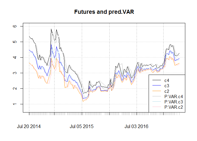
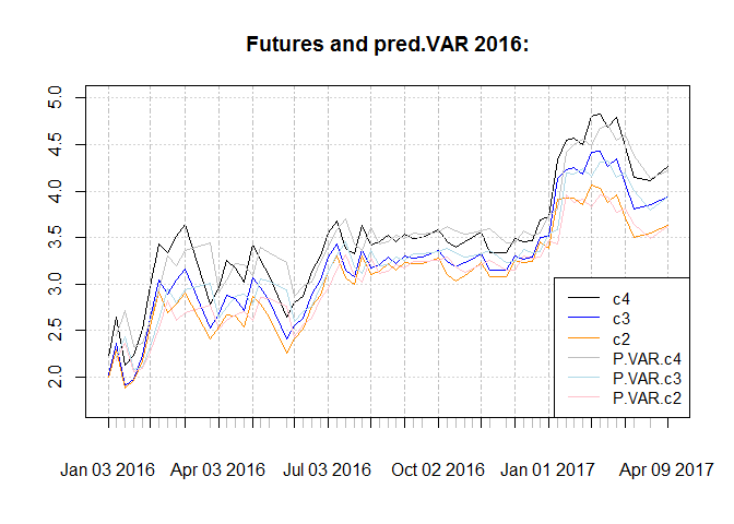
In sample RMSE for the contracts are as below. As we we RMSE is substantially lower for the sub sample.

## [1] "Whole sample"

	c2	c3	c4
RMSE	0.2158	0.2457	0.284

## [1] "2016 onward"

	c2	c3	c4
RMSE	0.179	0.2004	0.2283

The graph for spread of contracts and resulted spread from forecasts:

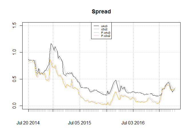
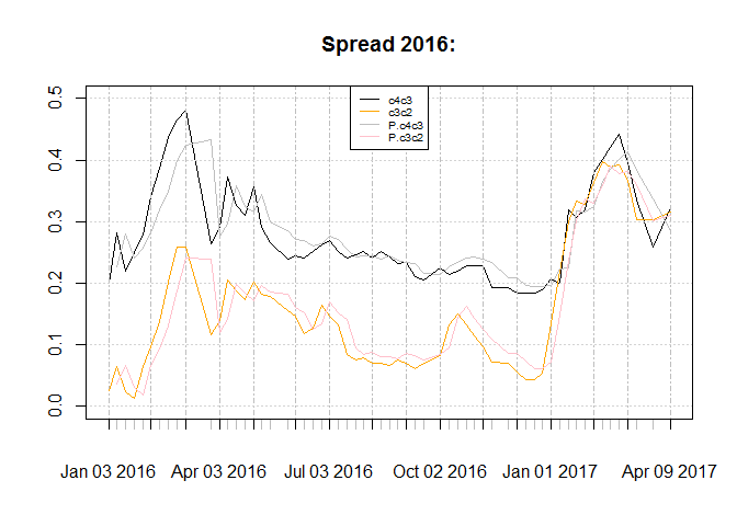
Unlike AFNS, reduced form follows the data on the fact that c2c3 spread is more than c4c3 spread. This is plausible :)

Step 2

For estimating $\hat{\rho}^Q , \hat{\delta}_1$ following function are needed:

power.mat<- function ( mat = rho , power = 8){
  out<- list()
  out[[1]]<- mat
  for ( i in 2 : power){
    out[[i]] <- out[[i-1]]%*%mat 
  }
  return(out)
}


b_n_fun<- function( rho = rho_i, delta_1 = rnorm(3), n = 8){
  delta_1<- abs(delta_1)
  out = list()
  for(i in 1 : n){
    
    sum_rho.power<- diag(3)
    if( i > 1){
      rho_sep<- rho[ c( 1 : (i-1))]
      for( j in 1 : length (rho_sep)){
        sum_rho.power<- sum_rho.power + t(rho_sep[[j]])
      }
    }
    out[[i]]<- (sum_rho.power %*% delta_1) * (1 / (i))
    
  }
  return(out)
}

Having them in hand we can numerically minimize step 2:

library(OpenMx)
pi2.g2.fun<- function (x1 = par, phi21star.hat. = phi21star.hat,
                       omega1.star.hat. = omega1.star.hat){
  
  rhoQ<- matrix( c( x1[1], 0, 0,x1[4] , x1[2], 0, 
                    x1[5:6], x1[3]), ncol = 3, byrow = TRUE)
  delta_1. <- x1[7:9]
  pnlt<- 0
  #if( x1[1] < x1[2] | x1[1] < x1[3] | x1[2] < x1[3]) pnlt<- .001
  
  rho_i<- power.mat(mat = rhoQ , power = 8)
  
  b_i<- b_n_fun(rho = rho_i, delta_1 = delta_1., n = 8)
  
  
  pi.hat_2<- cbind( c( c( phi21star.hat. %*% omega1.star.hat.), vech(omega1.star.hat.)))
  B_1<- rbind( t(b_i[[4]]), t(b_i[[6]]), t(b_i[[8]]))
  B_2<- t(b_i[[2]])
  g_2<- cbind( c( c( B_2 %*% t(B_1)),  vech(B_1 %*% t( B_1))))
  out<- t(pi.hat_2 - g_2) %*% (pi.hat_2 - g_2)
  out<- out + pnlt
  return(out)
}

par<- rnorm(9)
par.pi2.g2<- optim(par , pi2.g2.fun, phi21star.hat. = phi21star.hat, omega1.star.hat. = omega1.star.hat,
      control = list(maxit = 10000))$par

rhoQhat<- matrix( c( par.pi2.g2[1], 0, 0,par.pi2.g2[4] , par.pi2.g2[2], 0, 
                     par.pi2.g2[5:6], par.pi2.g2[3]), ncol = 3, byrow = TRUE)
rhoQhat_i<- power.mat(mat = rhoQhat , power = 8)
deltahat_1<-  par.pi2.g2[7:9]

b_i<- b_n_fun(rho = rhoQhat_i, delta_1 = deltahat_1, n = 8) 
Bhat_1<- rbind( t(b_i[[4]]), t(b_i[[6]]), t(b_i[[8]]))
Bhat_2<- t(b_i[[2]])

Here I used OpenMx package. I had expm package loaded and it wrote the following message :D :

”** Holy cannoli! You must be a pretty advanced and awesome user. The expm package is loaded. Note that expm defines %^% as repeated matrix multiplication (matrix to a power) whereas OpenMx defines the same operation as elementwise powering of one matrix by another (Kronecker power).”

I feel that they are pretty cool :)

Step 3

$\hat{\rho}$ is simply estimated as follows:

rhohat<- solve(Bhat_1)%*% phi11star.hat %*% Bhat_1

Step 4

For estimating $\hat{c}^Q and \hat{\delta}_0$$ I needed the following function:

a_n_fun<- function( b = b_i, delta_0 = rnorm(1), c_Q = rnorm(3), Sigma = diag(3), n = 8){
  
  out = list()
  for(i in 1 : n){
    
    sum_b<- delta_0
    out[[1]]<- sum_b
    sum_2<- 0 
    if( i > 1){
      b_sep<- b[ c( 1 : (i-1))]
      for( j in 1 : length (b_sep)){
        sum_b<- sum_b + t(b_sep[[j]]) * j
        sum_2<- sum_2 + ((i ^ 2) * ( t(b_sep[[j]]) %*% Sigma %*% t(Sigma) %*% b_sep[[j]]) )
      }
      out[[i]]<- ((sum_b %*% c_Q) * (1 / (i))) - (sum_2 / (2*n))
    }
    
    
  }
  return(out)
}

Then I minimized it to estimate the unknowns:

A.Ahat<- function( x2 = par, a_n_fun. = a_n_fun, b_i. = b_i, sigma_e. = sigma_e,
                   Bhat_1. = Bhat_1, Bhat_2. = Bhat_2, rhohat. = rhohat){
  
  a_n_l<- a_n_fun.( b = b_i., delta_0 = x2[1], c_Q = x2[2:4],
                    Sigma = diag(3), n = 8)
  A_1<- rbind( a_n_l[[4]], a_n_l[[6]], a_n_l[[8]])
  A_2<- a_n_l[[2]]
  
  LHS1<- (diag(3) - Bhat_1. %*% rhohat. %*% solve(Bhat_1.)) %*% A_1
  
  
  LHS2<- A_2 - Bhat_2. %*% solve(Bhat_1.) %*% A_1
  
  sum.sq.diff<- sum((A1star.hat - LHS1)^2) + ((A2star.hat - LHS2)^2)
  return(sum.sq.diff)
}


par<- rnorm(4)
par.A.Ahat<- optim( par , A.Ahat, b_i. = b_i, sigma_e. = sigma_e,
       Bhat_1. = Bhat_1, Bhat_2. = Bhat_2, a_n_fun. =a_n_fun,
       rhohat. = rhohat
       )$par

deltahat_0<- par.A.Ahat[1]
chat_Q<- par.A.Ahat[2:4]

a_n_l<- a_n_fun( b = b_i, delta_0 = deltahat_0, c_Q = chat_Q,
                  Sigma = diag(3), n = 8)
Ahat_1<- rbind( a_n_l[[4]], a_n_l[[6]], a_n_l[[8]])
Ahat_2<- a_n_l[[2]]

Results

The estimations for whole sample and sub sample are:

## [1] "Whole sample"

$\hat{\rho}^Q$ :

1.106 0 0

0.0222 -1.071 0

-1.733 2.146 -0.2297

$\hat{\delta}_1$ : 0.0001887, -0.9224 and 0.172
$\hat{B}_1$ :

-0.2029 0.07062 0.03488

-0.246 0.03973 0.02331

-0.2863 0.02335 0.01749
$\hat{B}_2$ :

-0.1387 0.1519 0.06626
$\hat{\rho}$ :

1.106 0 0

0.0222 -1.071 0

-1.733 2.146 -0.2297
$\hat{\delta}_0$ : 24.57
$\hat{c}^Q$ : -2.373, 45.97 and -45.26
$\hat{A}_1$ :

8.423

11.53

11.64
$\hat{A}_2$ :

-3.28

## [1] " 2016 onward"

$\hat{\rho}^Q$ :

-0.9431 0 0

2.055 0.2597 0

-0.4237 -0.3477 -1.118
$\hat{\delta}_1$ :-1.367, 0.4522 and 2.122
$\hat{B}_1$ :

0.1 -0.06354 -0.1409

0.1218 -0.0589 -0.1592

0.1378 -0.05961 -0.1805
$\hat{B}_2$ :

0.05392 -0.08404 -0.1252
$\hat{\rho}$ :

-0.9431 0 0

2.055 0.2597 0

-0.4237 -0.3477 -1.118
$\hat{\delta}_0$ :-1.802
$\hat{c}^Q$ :42.03, 18.91 and 147.3
$\hat{A}_1$ :

-76.94

-56.22

-55.09
$\hat{A}_2$ :

-166.4

Conclusion

Since gold coin futures have no convenience yield and since interest rate is constant in Tehran market, I thought that using interest rate model for term structure of gold coin futures in Tehran market is reasonable. While the last two models were not satisfactory, it seemed to me that latent factor model is kinda cool for this matter. Well the whole interpretation procedure needs to be changed if this model is going to be used, and since I just do these things for fun, I would not do it here :)

Term Structure Of Gold_coins Part 3

Latent Factors