Why an interest rate model for future?
In last post, we saw that since gold coins are useless, convenience yield is almost zero for gold coin futures. Furthermore since interest rates are almost constant in Tehran market and the are treated as external variables that are determined by central bank. Putting aside interest rate and convenience yield, the models for future term structure could reduce to processes like interest rate. Literally using the same names as the names of the models for the later, is not correct, because we are using it in a different context, yet I prefer to not change the names. So we are using wrong models for right reasons. It is possible that the results become cat-astropic, like a cat that is plotting against hooman :)
CIR
Given the P dynamics by completely affine here ans here, using Kalman filter for estimation, and by looking at this matlab code by the later, I used the following function for estimation:
CIR.fun<- function (p, # parameters
                    Y, # series
                    tau # delta t
                    ){
  theta  = p[1]
  kappa = p[2]
  sigma = p[3]
  lambda = p[4]
  sigmai = p[5:8]
  sigmai2 = sigmai^2
  R <- diag(sigmai2)
  dt <- 1/52
  C <- theta* ( 1 - exp( - kappa*dt))
  H <- exp(-kappa*dt)
  gamma<- sqrt((kappa+lambda)^2+2*sigma^2)
  logAi<- (2 * kappa * theta / ( sigma^2))*log( (2 * gamma*exp(( gamma + kappa + lambda) * tau / 2))/
                                                  (2*gamma + (gamma + kappa + lambda)*
                                                     ( exp( gamma * tau) - 1) ))
  Bi<- 2*(exp(gamma*tau)-1)/(2*gamma + (gamma+kappa+lambda)*
                               (exp(gamma*tau)-1))
  logAtho<- logAi/ tau
  Btho<- Bi / tau
  initx = theta
  initV = (sigma^2)*theta/(2*kappa)
  AdjS=initx
  VarS=initV
  LL<- rep(0, nrow(Y))
  CIR.pred<- matrix( NA, ncol = ncol(Y), nrow = nrow(Y))
  J<- 0
  for ( i in 1:nrow(Y)){
    PredS=C+H*AdjS
    Q=theta*sigma*sigma*(1-exp(-kappa*dt))^2/(2*kappa)+sigma*sigma/kappa*
      (exp(-kappa*dt)-exp(-2*kappa*dt))*AdjS
    VarS=H*VarS*H+Q
    PredY=logAi+Bi*PredS
    VarY=as.numeric(VarS) * (Bi%*%t(Bi))+R
    if( det( VarY) <= 10^(-14)){
      J <- 1
    } else {
    PredError=Y[i,] -PredY
    KalmanGain=as.numeric(VarS)*Bi%*%solve(VarY)
    AdjS=PredS+KalmanGain%*%t(PredError)
    VarS=VarS*(1-KalmanGain%*%(Bi))
    DetY=det(VarY)
    if (DetY <= 10^(-14)){
      J <- 1
    } else{
      J <- 0
      CIR.pred[ i,]<- PredY
    LL[i]=-(ncol(Y)/2)*log(2*pi)-0.5*log(DetY)-0.5*PredError%*%solve(VarY)%*%t(PredError)
    }
    }
  }
  if( J == 1){
    sumll <- 10^5
  } else {
  sumll=-sum(LL)
  }
  return(list( loglike = sumll, CIR.pred = CIR.pred))
}

p=c(0.10,0.05,0.075,-0.4,rep(.1, 4))
tau1 = c(2/12, 4/12, 6/12, 8/12)

spot.futures.scaled.2016<- spot.futures.scaled["2016-01-01::"]

par.CIR<- nmk(p, CIR.fun,
    control = list(maxfeval = 10000),
     Y = spot.futures.scaled[,2:5], tau = tau1, ll = TRUE)
par.CIR.2016<- nmk(p, CIR.fun,
    control = list(maxfeval = 10000),
     Y = spot.futures.scaled.2016[,2:5], tau = tau1, ll = TRUE)
results and graphs of the optimization for whole sample and the sample after 2016 are:
## [1] "Whole sample"
| theta | kappa | sigma | lambda | sigma1 | sigma2 | sigma3 | sigma4 |
|---|---|---|---|---|---|---|---|
| -1.527 | -0.005896 | 2.434 | 4.775 | 0.62 | 0.2043 | 0.001015 | 0.4187 |
## [1] "2016 onward"
| theta | kappa | sigma | lambda | sigma1 | sigma2 | sigma3 | sigma4 |
|---|---|---|---|---|---|---|---|
| 21.98 | 0.0048 | 3.155 | 14.64 | 0.07389 | 0.03085 | 0.1735 | 0.4474 |
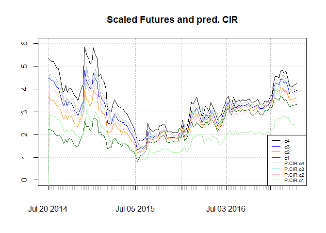 
As charts show, it fails to make account for slope. And structural break after 2016 is obvious. Since λ is positive and as a result market price of risk is negative, I will not consider CIR for this purpose.
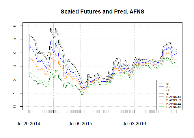
Affine Arbitrage-Free Nelson-Siegel (AFNS)
Given essentially affine structure the canonical P dynamics are given here. I would consider independent factor model. The code is available here, yet some minor changes are needed for our case. The optimization using nmk is:
## [1] "Whole sample"
| kappa11 | kappa22 | kappa23 | sigma11 | sigma22 | sigma33 | theta1 | theta2 |
|---|---|---|---|---|---|---|---|
| 6.985 | 0.8552 | 0.09665 | 0.8821 | 0.7551 | 8.65 | 2.154 | -0.5502 |
| theta3 | lambda | sigma1 | sigma2 | sigma3 | sigma4 |
|---|---|---|---|---|---|
| 2.302 | 0.5419 | 0.1355 | 0.01691 | 0.1362 | 0.02269 |
## [1] "2016 onward"
| kappa11 | kappa22 | kappa23 | sigma11 | sigma22 | sigma33 | theta1 | theta2 |
|---|---|---|---|---|---|---|---|
| 73.39 | 1.941 | 0.07133 | 0.4388 | 1.037 | 83.95 | -47.48 | 49.99 |
| theta3 | lambda | sigma1 | sigma2 | sigma3 | sigma4 |
|---|---|---|---|---|---|
| -97.41 | 0.03821 | 4.179e-06 | 0.03697 | 0.002053 | 0.1554 |
Graphs and RMSE are:
## [1] "Whole sample"
| c1 | c2 | c3 | c4 | |
|---|---|---|---|---|
| RMSE | 0.2464 | 0.2749 | 0.3727 | 0.4246 |
## [1] "2016 onward"
| c1 | c2 | c3 | c4 | |
|---|---|---|---|---|
| RMSE | 0.1672 | 0.209 | 0.2496 | 0.3779 |
Unlike CIR, AFNS can consider slope. The structural change is less obvious in the graphs, but looking at RMSE it shows that sub sample estimation shows an improvement. Considering sub sample there is a persistent under estimation for fourth contract. Since this contract is the most liquid one it is not plausible. Looking at graph we see a lag between shocks to contracts and their prediction, which is as far as I see before, is typical for this kind of models unless we have an external variable that can predict the shocks.
RMSE for in-sample four step ahead forecasts are:
## [1] "Whole sample"
| c1 | c2 | c3 | c4 | |
|---|---|---|---|---|
| RMSE | 0.4475 | 0.5045 | 0.6389 | 0.7453 |
## [1] "2016 onward"
| c1 | c2 | c3 | c4 | |
|---|---|---|---|---|
| RMSE | 0.3278 | 0.4253 | 0.5107 | 0.6927 |
Spread by AFNS
Lets see how spread and their prediction by ANFS looks like:
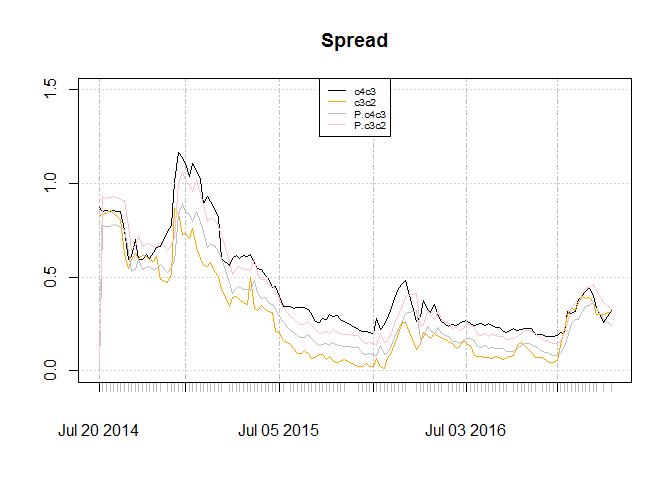
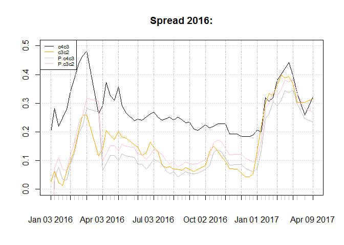
The spreads shows consistent over estimation and under estimation for each case. And it fails to include c3c2 being more than c4c1 which is temporary. Since model says it is a deviation it could use for trade yet the data is short for supporting this idea and the resulting profit dont seem to be much more than 10% risk free rate in this market. Considering sub sample, forecasts of c3c2 is better. Forecast of c4c3 shows a bump in middle of the chart that does not exist for the original series.