Introduction
I think that one of the most fascinating aspects of markets is term structure of instruments. I just love to see how highly correlated processes get affected by time. This property is of utmost beauty in my mind. During the time I was serving as a lieutenant, I had lots of spare time and I had the opportunity to read “Term-Structure Models, A Graduate Course” by Damir Filipovic. Now that I am in active search for a job, I have enough spare time to estimate some of the models of this book.
In Tehran, they have introduced futures on gold coins few years ago. I will try to fit some models on their term structure during next posts. In this post I try to see the basic properties and whether they behave as international markets.
About 15 months ago, I saw some obvious arbitrage opportunities in Tehran gold coin future market, especially in their spreads and butterflies. I had backtested strategies which yielded about 50 percent profit per year, yet by the time I wanted to use them, market had an structural change and the arbitrage get eroded. Being late in noticing something is not always good :) So in flowing posts I would consider data after 2016 for computations.
I saw the flowing considering gold coin future market:
- Latest contract is the most liquid one
- Nearest contract trading includes big slippage
- Curvature changes and seems to be mean reverting
- Before 2016 by having an inventory of cash or coin, arbitrage was existed
- there is no convenience yield on keeping gold coins, they are almost useless
- considering contracts, slope is almost always greater than zero . If we consider spot price, backwardation occurs.
- During late 2015 spread reached to zero.
Considering these, it is possible to use models on interest rate term structure on gold coins. So I will test them to see how well they are. Since these models are tested on simulations based on interest rate, I will change the range of the future contract to 1 to 10. Since I will focus on after 2016, I would not use shadow rates models.
Continius contracts and data
I got the data on contracts data from MofidTrader. Then I proportionally backward adjusted them. I used the same source for gold coin spot prices. for sake of comparability I also adjusted them by the ratios from the most liquid contract. Since we will use increments here that would not make a problem, and comparison would be easier.
library(xts)
date_t<- paste( coin$DAY, coin$HOURE)
date_t<- as.POSIXct( date_t)
xts.coin<- as.xts( coin[,-c( 1:2)], order.by = date_t)

date_t<- paste( Future_4$DAY, Future_4$HOURE)
date_t<- as.POSIXct( date_t)
xts.Future_4<- as.xts( Future_4[,-c( 1:2)], order.by = date_t)

date_t<- paste( Future_3$DAY, Future_3$HOURE)
date_t<- as.POSIXct( date_t)
xts.Future_3<- as.xts( Future_3[,-c( 1:2)], order.by = date_t)

date_t<- paste( Future_2$DAY, Future_2$HOURE)
date_t<- as.POSIXct( date_t)
xts.Future_2<- as.xts(F uture_2[,-c( 1:2)], order.by = date_t)

date_t<- paste( Future_1$DAY, Future_1$HOURE)
date_t<- as.POSIXct( date_t)
xts.Future_1<- as.xts( Future_1[,-c( 1:2)], order.by = date_t)


spot.futures<- cbind(spot = to.daily( xts.coin$CLOSE)[,4] ,
                     c1 =  to.daily( xts.Future_1$CLOSE)[,4] ,
                     c2 =  to.daily( xts.Future_2$CLOSE)[,4] ,
                     c3 =  to.daily( xts.Future_3$CLOSE)[,4] ,
                     c4 =  to.daily( xts.Future_4$CLOSE)[,4])
colnames(spot.futures)<- c("spot", "c1", "c2", "c3", "c4")

spot.futures<- spot.futures[ complete.cases( spot.futures$c1 ),]
spot.futures<- spot.futures[ complete.cases( spot.futures$c4 ),]
spot.futures<- spot.futures[ complete.cases( spot.futures$c2 ),]
spot.futures<- spot.futures[ complete.cases( spot.futures$c3 ),]
spot.futures<- spot.futures[ complete.cases( spot.futures$spot ),]
spot.futures<- spot.futures[-( which( spot.futures$c3 == 0)),]


plot( spot.futures[,1], main = "spread", cex.main = 0.8, ylim = c(9500000, 16000000))
lines( spot.futures[,2],col=4)
lines( spot.futures[,3], col = 3)
lines( spot.futures[,4], col = 2)
lines( spot.futures[,5], col = 6)
abline( v = as.POSIXct( beg_days), col = 2, lty = 3 )
legend( "topright", legend = c("adj. spot", "c1", "c2", "c3", "c4"), col = c(1,4 ,3, 2, 6),
       cex = 0.8, lwd = c( 1, 1, 1, 1, 1))


library(plotly)
plot_ly( y = index( spot.futures), z = ~spot.futures) %>% add_surface()
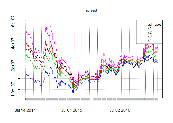
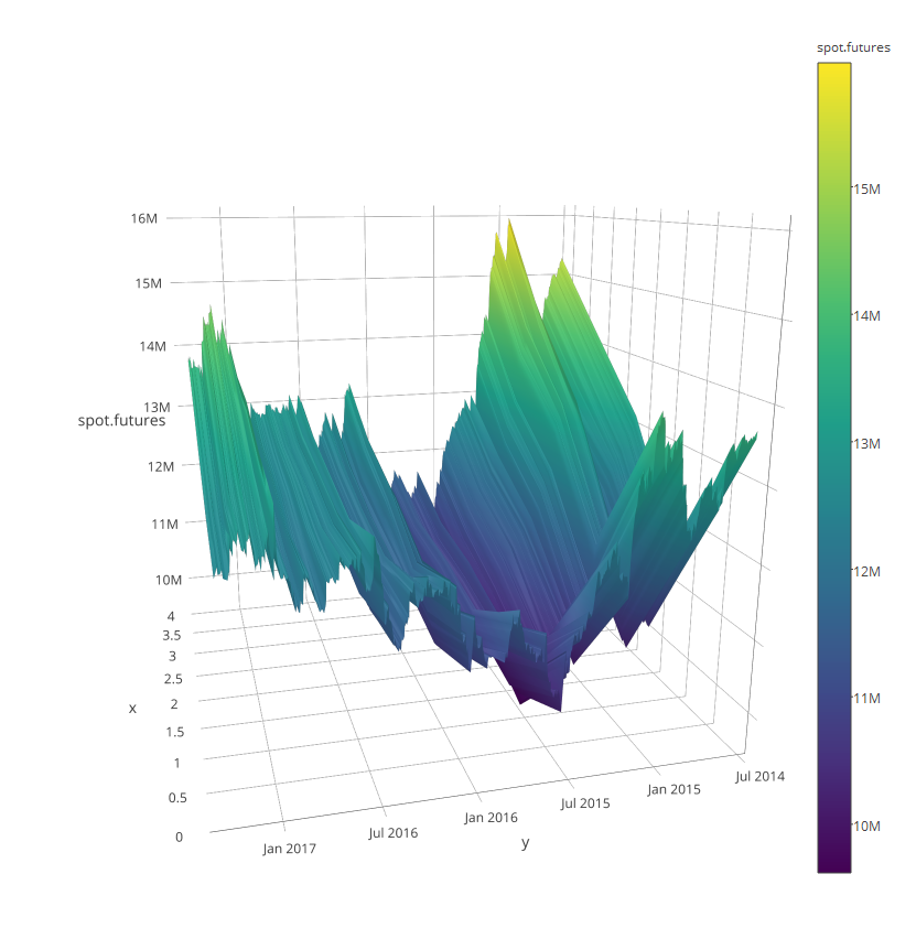
As we see at the end of 2015 there is negative rates and difference between contracts shows a structural change after 2016.
PCA and correlation
Lets see whether typical features of term structure occurs here or not.
path = "C:/Users/msdeb/Documents/Stock and trades/"
setwd(path)
load(".RData")


spot.futures.scaled<- (spot.futures - (min( spot.futures$spot, na.rm = TRUE) + 1) ) / sd(spot.futures$c4)

log.ret<- apply(as.data.frame(spot.futures.scaled["2016-01-01::"]), 2, function(x)  diff.xts(log(x)))

T1<- prcomp( log.ret[-1,1:5])
library(pander)
panderOptions("digits", 4)
pander(summary( T1)$importance)
| PC1 | PC2 | PC3 | PC4 | PC5 | |
|---|---|---|---|---|---|
| Standard deviation | 0.1527 | 0.02887 | 0.01439 | 0.008715 | 0.006069 |
| Proportion of Variance | 0.9528 | 0.03408 | 0.00847 | 0.0031 | 0.00151 |
| Cumulative Proportion | 0.9528 | 0.9869 | 0.9954 | 0.9985 | 1 |
pander( -T1$rotation)
| PC1 | PC2 | PC3 | PC4 | PC5 | |
|---|---|---|---|---|---|
| spot | 0.3492 | 0.9037 | 0.2448 | -0.02269 | 0.02893 |
| c1 | 0.516 | 0.02142 | -0.8206 | -0.2121 | -0.1221 |
| c2 | 0.461 | -0.1753 | 0.08519 | 0.8545 | -0.1391 |
| c3 | 0.4746 | -0.2757 | 0.2298 | -0.2091 | 0.776 |
| c4 | 0.4172 | -0.2757 | 0.4546 | -0.425 | -0.6022 |
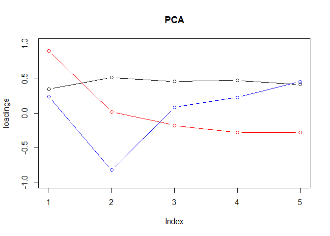
plot(-T1$rotation[,1], type = "b", ylim = c(-1,1), ylab ="loadings", main = "PCA")
lines(-T1$rotation[,2], type = "b", col = 2)
lines(-T1$rotation[,3], type = "b", col = 4)
pander(cor(log.ret[-1,1:5]))
| spot | c1 | c2 | c3 | c4 | |
|---|---|---|---|---|---|
| spot | 1 | 0.8811 | 0.8585 | 0.8434 | 0.8343 |
| c1 | 0.8811 | 1 | 0.975 | 0.9718 | 0.9587 |
| c2 | 0.8585 | 0.975 | 1 | 0.9876 | 0.981 |
| c3 | 0.8434 | 0.9718 | 0.9876 | 1 | 0.9905 |
| c4 | 0.8343 | 0.9587 | 0.981 | 0.9905 | 1 |
It seems to me that level, slope and curvature exits. Yet level looks a bit upward at the begining which is not very satisfactory. Also de-correlation occurs significantly.
Conclusion
Having seen that level and slope exist and considering that convenience yield is not existed, I would try to see performance of CIR, affine process estimation and affine arbitrage free nelson sigel term structure in the future posts.