Momentum
Few days ago I read Fact, Fiction and Momentum Investing and it made me curious to see how momentum investing works in Tehran Stock Exchange. Considering large inflation rate, I won’t imagine that short side of the momentum works well. Further, short selling is not possible.
Here I have not splitted stocks by size categories. Monthly data was used for computing the results. I used the following function for getting the names of the stocks to be sold and bought. It considers the backward window to be computed, whether considering the latest month or not, portion of the stocks to be considered based on volume (for liquidity reasons) and portion of the stocks to be long or short in portfolio.
z <- zoo(retDATAw, retDATAw$DATE)
t <- aggregate(z, as.yearmon, tail, 1)
retDATAw.mont <- as.data.frame(t)
retDATAw.mont <-  apply(retDATAw.mont , 2, function(x)
  as.numeric(coredata(x)))
retDATAw.mont <- as.data.frame(retDATAw.mont)
retDATAw.mont$DATE <- as.Date(index(t$DATE))
rm(z); rm(t)


names.momentum <- function(data = retDATAw.mont,
                           WDATA. = WDATA,
                           win.back = 12,  # backward window for computing return
                           win.start = 134,  # starting raw for computation
                           last.month = TRUE,  # whether to skip latest month
                           data_NA_rm. = data_NA_rm,
                           portion.mom = 3 / 10,  # portion of stocks to be short or long
                           n.var = 3 / 4    # portion of stocks to be considered based on volume
                           ) {
  DATE.end <- data$DATE[win.start]

  if (last.month == TRUE) {
    WDATA. <- subset(WDATA., WDATA.$DATE <= data$DATE[win.start] &
                       WDATA.$DATE > data$DATE[win.start - win.back])
    data <- subset(data, data$DATE <= data$DATE[win.start] &
                     data$DATE > data$DATE[win.start - win.back])
  } else{
    WDATA. <- subset(WDATA., WDATA.$DATE < data$DATE[win.start] &
                       WDATA.$DATE >= data$DATE[win.start - win.back])
    data <- subset(data, data$DATE < data$DATE[win.start] &
                     data$DATE >= data$DATE[win.start - win.back])
  }


  WDATA. <- ddply(WDATA., 'sym', .fun = function(x) data_NA_rm.(x),
          .progress = "tk")
  WDATA.$sym <- droplevels(WDATA.$sym)

  Ave_year_VOL <- summarise(group_by(WDATA., sym), mean = mean(VOL, na.rm = TRUE))
  Ave_year_VOL <- Ave_year_VOL[order(Ave_year_VOL$mean , decreasing  = TRUE), ]
  Ave_year_VOL <- as.data.frame(Ave_year_VOL)
  Ave_year_VOL[, 1] <- as.character(Ave_year_VOL[, 1])

  portion <- floor(n.var * dim(Ave_year_VOL)[1])
  portion <- as.numeric(portion)
  portion.sym <- c(Ave_year_VOL[(1:portion) , 1])

  data <- data[, (colnames(data) %in% as.factor(portion.sym))]
  period.ret <- ( data[dim(data)[1], ] - data[1, ]) / data[1, ]
  period.ret <- period.ret[order(period.ret , decreasing  = TRUE)]
  is.na.order <- apply(period.ret, 2, function(x)   sum(is.na(x)))
  period.ret <- period.ret[, which(is.na.order <= 0)]
  period.ret <- as.data.frame(names(period.ret))
  period.ret[, 1] <- as.character(period.ret[, 1])

  n.total <- dim(period.ret)[1]
  n.sym <- floor(portion.mom * n.total)

  names.long <- period.ret[1:n.sym,]
  names.short <- period.ret[((n.total - n.sym + 1):n.total),]

  out <- list(
      win.start = win.start,
      DATE = DATE.end,
      names.long = names.long,
      names.short = names.short
    )
  return(out)
}
After getting names of the stocks lets compute the returns:
SL.ret <- function(res = results,
                   retDATAw.mont. = retDATAw.mont) {
  weigths.long <-  matrix(0,
           ncol = dim(retDATAw.mont.)[2],
           nrow = dim(retDATAw.mont.)[1])
  weigths.short <- matrix(0,
           ncol = dim(retDATAw.mont.)[2],
           nrow = dim(retDATAw.mont.)[1])
  colnames(weigths.long) <- colnames(retDATAw.mont.)
  colnames(weigths.short) <- colnames(retDATAw.mont.)

  for (i in 13:191) {
    names.short <- res[[i]]$names.short
    names.long <- res[[i]]$names.long
    weigths.short[(i + 1), (colnames(names.short) %in% as.factor(names.short))] <-
      (1 / length(names.short))
    weigths.long[(i + 1), (colnames(weigths.long) %in% as.factor(names.long))] <-
      (1 / length(names.long))
  }
  weigths.short <- weigths.short[, -1]
  weigths.long <- weigths.long[, -1]

  group.data <- apply(retDATAw.mont.[, -1], 2, function(x)
    PerChange((x)))
  group.data[is.na.data.frame(group.data)] <- 0
  group.data <- 1 + group.data
  long.ret <- (diag((group.data[14:192, ]) %*% t(weigths.long[14:192, ])))
  long.ret <- as.xts(long.ret, retDATAw.mont.$DATE[14:192])
  short.ret <- diag((group.data[14:192, ]) %*% t(weigths.short[14:192, ]))
  short.ret <- as.xts(short.ret, retDATAw.mont.$DATE[14:192])
  out <- cbind(long.ret = long.ret, short.ret = -short.ret)
  return(out)
}

resoltat <- list()
for (i in 13:192)
  resoltat[[i]] <-
  names.momentum(
    win.start = i,
    last.month = TRUE,
    win.back = 12,
    n.var = 3 / 4
  )
momentum.12.L <- SL.ret(res = resoltat)
Results
I computed the results considering backward windows of 12, 6 or 3 months. For each one of them latest month is either included or excluded (in charts ‘L’ means excluded the latest month and the number stand for backward window period).
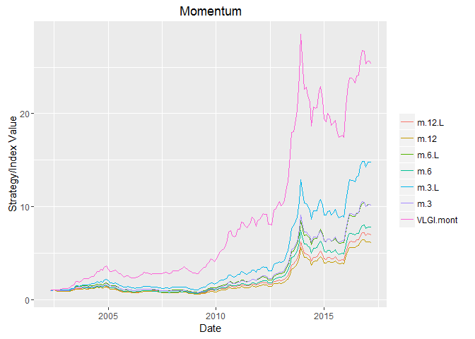
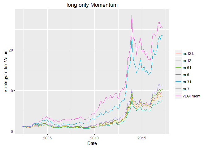
Conclusion
As I thought the short part of the momentum investing is not good for Tehran Stocks, the inflation just make it not reasonable. For the long part, except momentum with 3 month window that excludes last month (m.3.L), the rest both fails to catch with GDP deflator and VLGI. Even m.3.L shows less cumulative return than VLGI. And there exist a long four year and half draw-down duration in its chart which is not desirable. For this results I have not partitioned data by small vs. big. Since m.3.L was not so bad, I would try to consider it in the next post. I would try to get these data by Selenium when I got time( oh I don’t have a job yet, so I got the time and I’ll do it soon. Nowruz holidays are in few days, lets find some suitable strategies during that :)) ).