Benchmark Part III
Lets build mean variance portfolio and compare its out-of-sample forecasting power to VLGI. Since lots of discontinuities exist in the data and since the number of stocks grows over time I would use a variable basis, exactly like VLGI, that uses 3/4 of the most traded stocks during six month period preceding to the data.
For computing minimum variance portfolio, since there is no possibility to short stocks in Tehran Stock Exchange, I would use the criteria that no short is allowed. No leverage is another criteria that I would consider.
Data
I would use the same structure for data as before. For making matrix algebra easier I will change the shape of data.
source("C:/Users/msdeb/Documents/Stock and trades/functions.R")

retDATAw<- reshape( WDATA[, c( "DATE", "sym", "retCL_t")],
                   timevar = "DATE", idvar = "sym", direction = "wide")
retDATAw <- t( retDATAw)
colnames( retDATAw) <- retDATAw[1,]
retDATAw <- retDATAw[-1,]
J<- rownames( retDATAw)
J<- matrix( unlist( strsplit(J, split = "[.]")), ncol=  2,byrow = T)[, 2]
retDATAw<- apply( retDATAw, 2, function( x) as.numeric( x))
retDATAw<- as.data.frame( retDATAw)
retDATAw$DATE<- as.Date( J)
Quadratic Programming
For solving the quadratic optimization problem subject to our constraints I use solve.QP from “quadprog” package. Since data has lots of NAs there is a high probability that the resulting covariance function is not positive definite. In order to solve this problem I considered two solutions, first one is to use nearest positive definite matrix of covariance matrix. the second one is to use global Optimization by Differential Evolution. Former was computed by make.positive.definite function from “corocor” package, and second by “DEoptim” package.
Results with nearest positive definite matrix have less variance in the sample I used, and computing them are much less computationally expensive than DEoptim. So here I would write the results about the former. (I’m not perfectly familiar with parameter tuning of DEoptim, so maybe better results are available. For current mean variance optimization I think that nearest positive definite matrix will suffice, please tell me if you happen to know any other method and you think its more suitable, in advance thank you :) )
MV.ret<- function(data = train,
                  date_data. = date_data, NA_last_obs. = NA_last_obs,
         short = FALSE, min.mu = 0.001, ret.min = FALSE){
  date.beg<- as.Date( data$DATE[1])
 ith.break.date<- sum( date.beg >= date_data.)
 sub_index_data<- data[, ( colnames( data) %in% as.factor( portion.sym[[ ith.break.date]]))]
 sub_index_data<- droplevels( sub_index_data)
 win_length<- dim( sub_index_data)[ 1]
 sum.na.col<- apply( sub_index_data, 2, function(x) sum( is.na(x)))
 sub_index_data<- sub_index_data[, which( sum.na.col< (9*10))]

 mu.hat <- colMeans(sub_index_data, na.rm = TRUE)

 sigma2.hat <- cov( sub_index_data, use = "pairwise.complete.obs")
 m.sigma2.hat<- mean( sigma2.hat, na.rm = TRUE)
 sigma2.hat <- apply( sigma2.hat, 2, function(x) { x[(
   is.na( x))]<- m.sigma2.hat ; x})
 D.mat = 2 * sigma2.hat
 meq. = 1
 A.mat = cbind( rep( 1, dim( sigma2.hat)[ 1]),
                diag(dim(sigma2.hat)[1]))

 if( ret.min == TRUE & max( mu.hat) < min.mu ) {
   min.mu <- mean( mu.hat)
   print( " unattainable min.mu changed to avrerage mu.hat ")
 }

 if( short == TRUE & ret.min == FALSE) A.mat<- cbind(rep(1,dim(sigma2.hat)[1]))

 b.vec = c(1 , rep(0, dim( sigma2.hat)[1]))

 if( ret.min == TRUE & short == FALSE) {
   A.mat = cbind( mu.hat, rep( 1,dim( sigma2.hat)[1]),
                  diag(dim(sigma2.hat)[1]))
   b.vec = c( min.mu, 1 , rep( 0, dim( sigma2.hat)[1]))
   meq. = 2
 }

 if( ret.min == TRUE & short == TRUE) {
   A.mat = cbind( mu.hat, rep( 1,dim( sigma2.hat)[1]))
   b.vec = c( min.mu, 1)
 }

 sigma2.hat.PD<- make.positive.definite( sigma2.hat)
 D.mat = 2*sigma2.hat.PD

 qp.out = solve.QP( Dmat  =  D.mat,
                    dvec = rep(0, dim(sigma2.hat.PD)[1]),
                    Amat=A.mat, bvec=b.vec, meq= meq.)


 weig<- qp.out$solution
 weig[ abs( weig) < 1e-4]<- 0
 weig<- weig / sum( weig)


 retDATAw_last<- apply( sub_index_data, 2, NA_last_obs. )

 mu.p = crossprod (weig,mu.hat)
 sigma2.p= t( weig) %*%  sigma2.hat %*% weig
 ret.porfolio<- ( 1+ retDATAw_last[ dim (retDATAw_last)[1], ]) %*% weig
 out<- cbind ( mu.p = mu.p, sigma2.p = sigma2.p, ret.porfolio = ret.porfolio )
 colnames( out)<- c( "mu.p", "sigma2.p", "ret.portfolio")
 weig<- rbind( weig)
 colnames( weig) = colnames( sub_index_data)
 out<- cbind( out, weig)
 out<- cbind( out, date.beg)
 return(out)
}
solve.QP occasionally produces NaN, and I have not found any reasons for that ( replicating computations sometimes results in non NaN results), I use previous weights for computing the portfolio return in these cases.
MV.ret.prv<- function(d ata = train,
                  date_data. = date_data, NA_last_obs. = NA_last_obs,
                  weig = w.prv, date.beg = date.prv){
  ith.break.date<- sum( date.beg >= date_data.)
  sub_index_data<- data[, ( colnames(data) %in% as.factor( portion.sym[[ ith.break.date]]))]
  sub_index_data<- droplevels( sub_index_data)
  win_length<- dim( sub_index_data)[1]
  sum.na.col<- apply( sub_index_data, 2, function(x) sum( is.na( x)))
  sub_index_data<- sub_index_data[, which( sum.na.col< ( 9*10))]
  weig<- weig[ ( names( weig) %in% colnames( sub_index_data))]

  sigma2.hat <- cov( sub_index_data, use = "pairwise.complete.obs")
  m.sigma2.hat<- mean( sigma2.hat, na.rm = TRUE)
  sigma2.hat <- apply( sigma2.hat, 2, function(x) {x[( is.na( x))]<- m.sigma2.hat ; x})

  mu.hat <- colMeans( sub_index_data, na.rm = TRUE)
  weig[ abs( weig) < 1e-4]<- 0
  weig<- weig / sum( weig)

  retDATAw_last<- apply( sub_index_data, 2, NA_last_obs. )

  mu.p = crossprod  (weig, mu.hat)
  sigma2.p= t( weig) %*%  sigma2.hat %*% weig
  ret.porfolio<- ( 1+ retDATAw_last[ dim ( retDATAw_last)[1], ]) %*% weig
  out<- cbind ( mu.p = mu.p, sigma2.p = sigma2.p, ret.porfolio = ret.porfolio )
  colnames(out)<- c( "mu.p", "sigma2.p", "ret.portfolio")
  weig<- rbind( weig)
  colnames(weig) = colnames( sub_index_data)
  out<- cbind( out, weig)
  out<- cbind( out, date.beg)
  return(out)
}


win=120
n = dim( retDATAw)[1] - win + 1
fcmat = NULL
fit = NULL
  for(i in 130 : n)   {
    train <- retDATAw[ i:( i + win -1 ),]
    fit <- MV.ret( train, date_data. = date_data, NA_last_obs. = NA_last_obs,
                  short = FALSE, min.mu = 0.001, ret.min = FALSE)
    if( is.nan( fit[1,1]) != TRUE) {
      w.prv = fit[, 4 : ( length(fit) - 1)]
      date.prv = fit[ , length(fit)]
    }
    if( is.nan( fit[1,1])) {
      fit <- MV.ret.prv( data = train, date_data. = date_data,
                         NA_last_obs. = NA_last_obs,
                         weig = w.prv, date.beg = date.prv)
    }
      fit<- ( fit[,1:3])
      names.fit<- names( fit)
      fit<- rbind.data.frame( fit)
      colnames( fit)<- names.fit
      fit$DATE <- retDATAw[ (i + win -1) ,]$DATE
      fcmat<- rbind( fcmat, fit)
  }
This is how cumulative product of returns looks like:
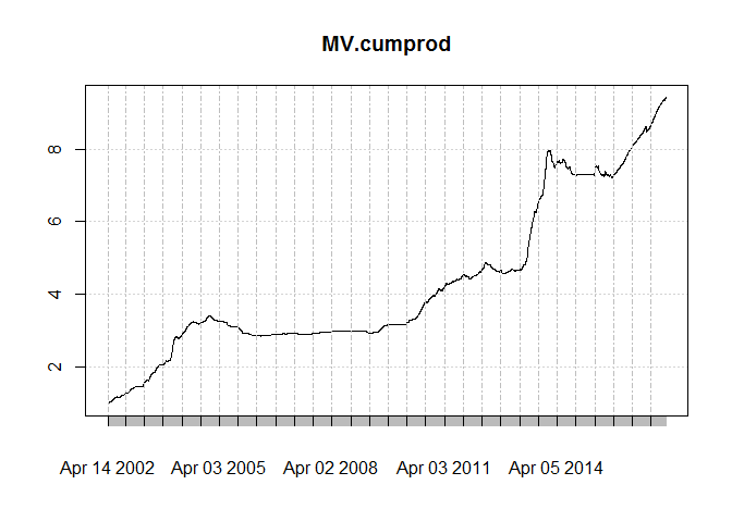
It seems to me that the results are pretty much inferior to Iran’s GDP deflator. That is to say even inflation is not covered under this portfolio, who dares to talk about idiosyncratic risk! Anyway, my objective was to compare its predictory power so lets see that.Like before I would use ri, t = α + β1ri, t − 1 + β2rm, t − 1 + e for getting errors.
th= floor((Sys.Date() - as.Date("2014-03-21"))*240/365)
h<-1
Order<-c(1,0,0)
dimmodel<-3
win=120
model="pARp"
regressed="retCL_t"
reg.type = "prd"
MAR_MOD.="ret.portfolio"
fcmat$ret.portfolio<- fcmat$ret.portfolio -1
######

WDATA.<- subset(WDATA, WDATA$DATE >= fcmat$DATE[1])
cl = createCluster(12, export = list("Arima.prd.IND",
                                     "reg.type",
                                     "h","Order","fcmat",
                                     "win", "th", "h","MAR_MOD.",
                                     "model","dimmodel","regressed"
),
lib = list("forecast", "dplyr"))


pARp.DIND.var<-ddply(.data = WDATA., .(sym), .progress= "tk",
                     .parallel = TRUE,
                     .fun =function(x) Arima.prd.IND(xsym = x,
                                                     MAR_MOD=MAR_MOD.,
                                                     KK=fcmat,
                                                     h=1,win=120, th=th, Order=c(1,0,0), model="pARp",
                                                     dimmodel=3, regressed="retCL_t",reg.type = "prd"
                     ))


stopCluster(cl)
Results
Out-of-sample 1 period ahead RMSE of VLGI is lower than mean variance method.
| RMSE MV | RMSE VLGI |
|---|---|
| 0.02374 | 0.02308 |
Lets see how rolling mean of the errors behave. Since square root is a concave function and I want to take mean for all the sample for each day, I would use Mean Absolute Error, MAE, instead. otherwise taking two mean and a square root between them would not result what we want due to Jensen inequality.
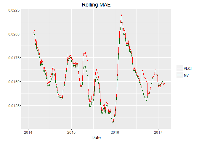
Plot shows that MV predict worse when errors increasing. Yet at the right part it produce slightly better result than VLGI.
Conclusion
Having all methods, hereafter I think using VLGI as a predictory variable seems better than others. So I would use that as my benchmark.