Benchmark Part II
For Constantly Rebalanced Portfolio (hereafter CPR) same distribution of
weights is used for all periods. Since CPR uses all the available data,
it is a rather omniscient benchmark that uses least effort. I use
monthly returns to compute the optimal weights for CPR wealth factor in which m is number
of stocks and wis are their respective weight.
Since newly introduced stocks are numerous I use the same method as before for computing 3/4 most traded stocks for the six month period ended at “2014-03-21” as the basis for computation.
Preparing data like previous post and getting monthly returns. Then changing its shape to wide form so matrix algebra becomes a lot easier:
source("C:/Users/msdeb/Documents/Stock and trades/functions.R")

# replacing NA with last observation
WDATA_last<- ddply(WDATA, .(sym), colwise(NA_last_obs,
                                          c("CLOSE", "retCL_t", "VOL")))

WDATA_last$DATE<- WDATA$DATE

# subseting data and finding most traded stocks
date_data<- c(seq.Date(from = as.Date("2001-03-21"), to = Sys.Date(), by = "2 quarter"), Sys.Date())

sub_year_data<- list()
for(i in 2: length(date_data)){
  sub_data<- subset(WDATA, WDATA$DATE < date_data[i] & WDATA$DATE >= date_data[i-1])
  sub_year_data[[i-1]]<- ddply(sub_data, 'sym', .fun = function(x) data_NA_rm(x), .progress = "tk")
}

portion.sym<- llply(sub_year_data, function(x) sort_base_index(x, n.var = 3/4))


sub_index_data<- WDATA_last[WDATA_last$sym %in% as.factor(portion.sym[[26]]),]
sub_index_data<- sub_index_data[ complete.cases(sub_index_data$CLOSE),]
sub_index_data<- subset(sub_index_data , sub_index_data$DATE >= date_data[27])
date_month<- c(seq.Date(from = as.Date("2001-03-21"), to = Sys.Date(), by = "month"), Sys.Date())

# monthly data: end of month
sub_data.month<- sub_index_data[(sub_index_data$DATE %in% date_month),]
sub_data.month<- droplevels(sub_data.month)
# computing monthly returns
t<- dlply(sub_data.month, 'sym', function(x) PerChange((x$CLOSE)))
sub_data.month$ret.month<- unlist(t)
rm(t)

# Reshaping data
retDATAw<- reshape(sub_data.month[,c(1,5,6)], timevar = "DATE", idvar = "sym", direction = "wide")
retDATAw <- t(retDATAw)
colnames(retDATAw) <- retDATAw[1,]
retDATAw <- retDATAw[-1,]
J<- rownames(retDATAw)
J<- matrix(unlist(strsplit(J, split= "[.]")), ncol=3,byrow=T)[,3]
retDATAw<- apply(retDATAw,2, function(x) as.numeric(x))
# removing first NA introduced by differencung
retDATAw<- retDATAw[-1,]
By next function I find the optimal weights for CPR. Since number of variables are more than 250, I increase the number of iterations for optim function.
CPR_weights<- function(data = retDATAw, w = weigths){
  w <- w/sum(w)
 portfo_return<- (1 +retDATAw) %*% w
 CPR_return<- cumprod( portfo_return)
 CPR_return<- CPR_return[ length( CPR_return)]
 weight_penalty<- (10000* (1 - sum( w))) ^ 2
 negative_penalty<- -sum( w[ w < 0])
 obj<- -(CPR_return) + weight_penalty + negative_penalty
 return( obj)
}

opt_CPR<- optim(  par = c(rep(1, 262)), CPR_weights, data = retDATAw, method  = "L-BFGS-B",
             lower   = 0, control = list(maxit = 1000),
             upper   = 1)


path = "C:/Users/msdeb/Documents/Stock and trades/"
setwd(path)
save.image()
Since inflation is high, the term w <- w/sum(w) need to be there so
the objective function won’t seek UFOs in the sky :) If we use cumsum
instead of cumprod there would be no need for that term.
Then weights for optimal CPR, equal weights for CPR are computed and related returns are computed. I also computed VLGI for comparisons.
w<- opt_CPR$par/sum(opt_CPR$par)
portfo_return<- (1 +retDATAw) %*% w
CPR_return<- cumprod( portfo_return)
CPR_return<- as.xts(CPR_return, order.by = as.Date(J[-1]))


w.equal<- c(rep(1/262, 262))
portfo_return.equal<- (1 +retDATAw) %*% w.equal
CPR_return.equal<- cumprod( portfo_return.equal)
CPR_return.equal<- as.xts(CPR_return.equal,
                          order.by = as.Date(J[-1]))

WDATA_last$r.C<- ddply(WDATA, .(sym), colwise(ratio.close, c("CLOSE")))[,2]
WDATA_last$DATE<- as.Date(WDATA$DATE)
index.VLGI<- index.maker(WDATA. = WDATA, WDATA_last. = WDATA_last)
index.VLGI<- as.data.frame(index.VLGI)
index.VLGI$DATE <- as.Date(index.VLGI$DATE)
index.VLGI<- as.xts(index.VLGI$VLGI, order.by = index.VLGI$DATE)
colnames(index.VLGI)<- c( "VLGI")
Results
The results for optimal CPR weights are:
##        Aluminum R.-a Cultur.Herit. Inv.-a     Dr. Abidi Lab.-a
##          0.027529633          0.185255685          0.559913093
##    Parsian Oil&Gas-a         Saipa Azin-a
##          0.218565318          0.008736271
It is interesting that among 262 stocks just 5 of them get chosen and future just 4 of them have weights more than 1 percent. (I ve seen anomal volumes in first two and forth one, maybe this could explain it, yet this is a in-sample analysis. For furthure analysis I need to change it to an out-of-sample one, if again these companies exist then the anomalities could be partly exlained)
Lets see how the plots for daily rebalanced portfolio by the optimal CPR monthly weights look. Values for VLGI are divided by its value at first day and multiplied by first value of optimal CPR so we have the same scale.
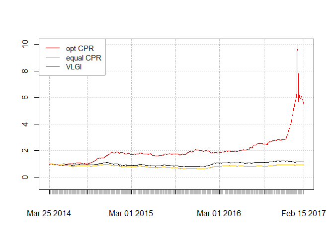
Contrary to my expectations, equal weight CPR is worse than VLGI. Optimal CPR generally have better results than VLGI. It also suffers from very sharp drawdown at the end of the chart. Its derivation could be result of sharp increase at the end of chart so if we use out-of-sample computations another set of weights would be computed.
If I use Optimal CPR as a benchmark, I think the results would be depressive :)) , for sure I cannot beat that, but it could be a good to compare with it, so I would have an eye on it. Before that I need to make it semi online, or compute it with predictory purposes. I would do that in another post.