Clustering
I saw that some stocks with industry similarities, like sugar industry or auto-makers, behave in a different manner than other stocks. Tehran Stock Exchange provide many different sub-indexes. Some of them have only handful of companies. As a way to deal with this matter, I prefer to use cluster analysis. Since I don’t want the number of each group to be similar, I would not use k-means. I would rather use hierarchical clustering using Ward method.
Having used ward method, first I would consider number of clusters, varying between 1 to 7 and take the one with the least out-of-sample rolling RMSE. Then I would consider different kind of distances to find which one results better results with the same criterion.
I had expect that 3 clusters with Malinowski distances less than 1 ( Lpnorms , before this post I was using p = 0.7, so the outliers would be less influential in clustering results), yet the results ,to my surprise, yielded different outcomes.
Clusters and indexes for each
Making data like previous post we use the following for estimating clusters and groups:
retDATAw<- reshape(WDATA_last[, c(1,2,5)], timevar = "DATE",
                   idvar = "sym", direction = "wide")
retDATAw <- t(retDATAw)
colnames(retDATAw) <- retDATAw[1,]
retDATAw <- retDATAw[-1,]
J<- rownames(retDATAw)
J<- matrix(unlist(strsplit(J, split= "[.]")), ncol=2,byrow=T)[,2]
rownames(retDATAw)<- J
rm(J)
retDATAw<- apply(retDATAw,2, function(x) as.numeric(x))
# scaling data
scale_retDATAw<- apply(retDATAw,2, scale)
# computing distances
distance<- dist(t(retDATAw), method = "minkowski", diag = TRUE, p =1)
distance<- as.matrix(distance)
for( i in 1:dim(distance)[1]){
  distance <- distance[,complete.cases(distance[i,]) ]
  distance <- distance[complete.cases(distance[,i]), ]
}
rm(i)
distance<- as.dist(distance)
# fitting cluster
fit = hclust(distance, method = "ward")


# finding number of cluster that has at least 5 members
n.groups.finder <- function(n.groups.) {
  success <- FALSE
  i <- 1
  n.groups <- n.groups.
  while (!success) {
    groups<- cutree(fit, n.groups)
    success <- sum(summary(as.factor(groups)) <= 5) < i
    i <- i + 1
    n.groups <- n.groups + 1
  }
  return(groups)
}

# cutting tree
cluster.results<- list()
for( i in 2 : 7){
n.groups <- i
groups <- n.groups.finder( n.groups)
n.gr<- which( summary(as.factor( groups))> 5)
cluster.results[[ i]]<- list( n.gr = n.gr, groups = groups)
}

# getting names of members
groups<- list()
temp<- list()
for( i in 2: length( cluster.results)){
  Cl.gr<- cbind( cluster.results[[i]]$groups)
  Cl.gr<- cbind.data.frame( groups = Cl.gr,sym = ( rownames( Cl.gr)))
  for( j in 1: length( cluster.results[[i]]$n.gr)){
    temp1<- Cl.gr[Cl.gr$groups== cluster.results[[i]]$n.gr[j],][,2]
    temp1<- droplevels(temp1)
    temp[[j]]<- temp1
}
  groups[[i]]<- temp
}
Here I used Whole sample for estimating clusters, this is against crossvalidation methods, since the data have lots of NA and because of that computing distances with rolling window was not possible, I used this method. I used this method with 3 cluster before and Temporal graph of clusters varies a lot during time. Now that the we get the name of members for each group we can make indexes for each of them. Using last posts results we have:
index.maker<- function(WDATA. = WDATA, date_data. = date_data,
                       sort_base_index. = sort_base_index,
                       WDATA_last. = WDATA_last, data_NA_rm. =data_NA_rm){

  sub_year_data<- list()
  for(i in 2: length(date_data.)){
    sub_data<- subset(WDATA., WDATA.$DATE <= date_data.[i] & WDATA.$DATE >= date_data.[i-1])
    sub_year_data[[i-1]]<- ddply(sub_data, 'sym',
                                 .fun = function(x) data_NA_rm.(x), .progress = "tk")
  }

  portion.sym<- llply(sub_year_data, function(x) sort_base_index.(x, n.var = 3/4))

  index_ave<- NULL
  last.VLIA<- 1
  last.VLIC<- 1
  for(i in 2 : (length (date_data.) -1)){
    sub_data<- subset(WDATA_last., WDATA_last.$DATE <= date_data.[i+1] &
                        WDATA_last.$DATE >= date_data.[i])
    sub_index_data<- sub_data[sub_data$sym %in% as.factor(portion.sym[[i-1]]),]
    dates.sub<- as.Date(levels(as.factor(sub_index_data$DATE)))
    VLIC<- cbind(c(rep(NA, (length(dates.sub) + 1))), c(rep(NA, (length(dates.sub) + 1))))
    VLIC[ 1, 1]<- last.VLIC
    for ( j in 2: (length(dates.sub) + 1)) {
      sub_index_data_date<- subset(sub_index_data, sub_index_data$DATE == dates.sub[j-1] )
      VLIC[j,]<- cbind(VLGI(sub_index_data_date$r.C, VLIC[ j - 1, 1]), as.Date(dates.sub[j-1]))

    }
    temp<- VLIC

    last.VLIC<- VLIC[ dim(VLIC)[1], 1]
    index_ave<- rbind(index_ave, temp)
  }
  index_ave<- index_ave[ complete.cases(index_ave[ ,2]),]
  colnames(index_ave)<- c("VLGI", "DATE")
  return(index_ave)
}


index.VLGI.groups<- list()
for ( i in 2: length( groups)){
  index.VLGI<- NULL
  for( j in 1: length(groups[[i]])){
    group.data<- subset( WDATA, WDATA$sym %in% groups[[i]][[j]])
    group.data_last<- subset( WDATA_last, WDATA_last$sym %in% groups[[i]][[j]])
    temp<- index.maker(WDATA. = group.data, WDATA_last. = group.data_last)
    temp<- cbind( temp, j)
    index.VLGI<- rbind(index.VLGI, temp)
  }
  index.VLGI.groups[[i]]<- index.VLGI
}

# computing reults for whole sample
index.VLGI.groups[[1]]<- cbind(index.maker(WDATA. = WDATA, WDATA_last. = WDATA_last),1)
Computing results
Using previously named function, we parallel compute the results for predictory autoregressive model ri, t = α + β1ri, t − 1 + β2rm, t − 1 + e :
th= floor((Sys.Date() - as.Date("2014-03-21"))*240/365)
h<-1
Order<-c(1,0,0)
dimmodel<-3
win=120
model="pARp"
regressed="retCL_t"
reg.type = "prd"
MAR_MOD.="DVLGI"


pARp.DVLGI.gr<- list()
for( i in 2: length(index.VLGI.groups)){
  VLGI.gr.data<- as.data.frame(index.VLGI.groups[[i]])
  colnames(VLGI.gr.data)<- c( "VLGI", "DATE", "gr")
  VLGI.gr.data$DATE<- as.Date( VLGI.gr.data$DATE)
  pARp.DVLGI<- NULL
  for( j in 1: length(levels(as.factor(VLGI.gr.data$gr)))){
    VLGI.data<- subset(VLGI.gr.data, VLGI.gr.data$gr == j)
  group.data<- subset( WDATA, WDATA$sym %in% groups[[i]][[j]])

  TIND.var<- cbind.data.frame(DATE = VLGI.data$DATE,
                              PerChange(VLGI.data$VLGI))
  TIND.var[is.nan.data.frame(TIND.var)] <- 0
  TIND.var[,2][ TIND.var[,2] == -Inf | TIND.var[,2] == Inf] = 0
  colnames(TIND.var)<- c("DATE", "DVLGI")

  group.data<- subset(group.data, group.data$DATE >= TIND.var$DATE[1])
  group.data$sym <- droplevels(group.data$sym)

  cl = createCluster(12, export = list("Arima.prd.IND", "group.data",
                                       "reg.type",
                                       "h","Order","TIND.var",
                                       "win", "th", "h","MAR_MOD.",
                                       "model","dimmodel","regressed"
  ),
  lib = list("forecast", "dplyr"))


  temp<-ddply(.data = group.data, .(sym), .progress= "tk",
                       .parallel = TRUE,
                       .fun =function(x) Arima.prd.IND(xsym = x,
                                                       MAR_MOD=MAR_MOD.,
                                                       KK=TIND.var,
                                                       h=1,win=120, th=th, Order=c(1,0,0),
                                                       model="pARp",
                                                       dimmodel=3, regressed="retCL_t",
                                                       reg.type = "prd"
                       ))

  stopCluster(cl)
  pARp.DVLGI<- rbind( pARp.DVLGI, temp)
  }
  pARp.DVLGI.gr[[i]]<- pARp.DVLGI
}
I do the same thing for whole sample without clusters too, so I could compare the results.
Number of cluster results
The results after “2016-01-01” shows that having four clusters has less rolling RMSE than others.
| 1 | 2 | 3 | 4 | 5 | 6 | 7 | |
|---|---|---|---|---|---|---|---|
| RMSE.gr | 0.0249 | 0.0249 | 0.02492 | 0.02478 | 0.02479 | 0.02482 | 0.0248 |
Distances
Having seen the results for number of clusters, I choose different distances for computing the results.
distance.seq<- c(.4,.5,.6,.7,.8,.9,1,1.5,2,3,4,6)
As I said before, I was choosing .7 as my p, but after seeing this I saw that Elucidian distance yields better results. Since we normalized returns for this computations, this means that Elucidian distance is approximately equal to 2(1 − ρ) in which ρ stands for correlation. So using correlations as a base for distances would have resulted the same thing. It is interesting that here, my phobia about including outliers are false :)) A very good step for overcoming my phobias experimentally :))
| 0.4 | 0.5 | 0.6 | 0.7 | 0.8 | 0.9 | 1 | 1.5 | |
|---|---|---|---|---|---|---|---|---|
| RMSE.dist | 0.02477 | 0.02481 | 0.02477 | 0.02467 | 0.02488 | 0.02488 | 0.02478 | 0.02472 |
| 2 | 3 | 4 | 6 | |
|---|---|---|---|---|
| RMSE.dist | 0.02267 | 0.02271 | 0.02275 | 0.02272 |
Conclusion
The results show that having four number of clusters with Elucidian distances yield better out-of-sample rolling RMSE results. So my guesses that some groups of stocks behave differently is not rejected under this criterion. But my idea about inclusion of outliers is rejected. Although I have not printed the groups since they are very lengthy, We would see more similar companies when p is less than one, yet the results are worse. When p is less than one one cluster is about auto-makers, and one include pharmaceutical industries (previously I saw sugar industry), but with Eluciden distance, results are more mixed, and number of members are much more. But we can see that most petrochemicals and petroleum companies are in the same cluster with some other companies of which some are like them and export oriented and revived after lifting the sanctions( group 1, 90 members.) And Auto-makers with some other not related companies are in another one( Group 2, 132 members.) Last group have more than 170 members and pharmaceutical and financial corporations are mostly inside that( group 4.)
The plot for the sub-indexes are like this:
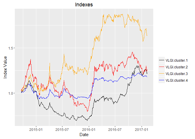
Looking at the graph is very interesting, and we see partly different and partly similar movements among groups. What is very fearsome is those movements that are common and very sharp, these could easily destroy my retirement plans. If I see more clearly, I see that these movements are mostly external and international shocks, like sanctions or lifting them or any expectations about them. I would write the next post about how to partly hedge these risk with existed instruments, oh yeah, I talked about instruments, but there is no options, Forex futures and short selling of stocks possible in this market and I have no access to international markets. I would try my best and cross my fingers for that, Voila!