Benchmark
Before anything get done, I need a benchmark to compare any performance to it. Tehran Stock Exchange provide numerous indexes which could be used for this sense. Seeing their definitions two things catches my eyes, first they use weights based on company size and second using data that are not adjusted for dividends which would result an inflated index. Another important thing is that Tehran Stock Exchange provides lots of groups indexes, some containing only a few companies as their base group.
What I need from a benchmark is that it provide better out-of-sample results, in other words I do not need a barometer for economic performance. What I want is predictory power or a sensible portfolio and the results would be tested in this sense. For reaching to this objective I have several things in my mind that I would test them:
- Creating indexes and compare them to existed indexes
- Price based indexes
- Indexes like Value Line Composite
- Mean-Variance portfolio
- Constant Rebalanced Portfolio
Absence of predetermined logical groups made me to consider cluster analysis for grouping stocks and building related indexes too, I will consider it in another post.
Creating Indexes
For creating indexes I take into account the next two observation. Firstly there are some companies that are not liquid at all and second, the number of stocks in the market has increased from about 110 to , 440 during 16 years. So I consider 3/4 of stocks that have higher volume during last period and I change the basket every six months form “2001-03-21”. In another way we could fix the number of stocks as our base I chose the six months ending at “2014-03-21” as the base for index. Adjusted prices is used for this computations. Another interesting feature of Tehran Stocks data is that they could be not been allowed for trading for a considerable amount of time. For solving this problem when I created the data I excluded the stocks that have not traded for the last 7/10 trading days for each subset. For these matters following functions are used for this:
library(plyr)
library(dplyr)
library(xts)
library(data.table)
library(forecast)

date_data<- c(seq.Date(from = as.Date("2001-03-21"), to = Sys.Date(), by = "2 quarter"), Sys.Date())

data_NA_rm<- function(x){
if(sum(is.na(x$CLOSE)) >= (7/ 10)*dim(x)[1]){
  temp <- NULL
  } else {
    if(var(x$CLOSE, na.rm = TRUE) == 0) {temp <- NULL} else {
      temp <- x
    }
  }
  return(temp)
}


# subsetting data
sub_year_data<- list()
for(i in 2: length( date_data)){
sub_data<- subset( WDATA, WDATA$DATE <= date_data[i] & WDATA$DATE >= date_data[i-1])
sub_year_data[[i-1]]<- ddply( sub_data, 'sym', .fun = function(x) data_NA_rm(x), .progress = "tk")
}

# Sorting stocks based on VOL
sort_base_index<- function(x, # data
                           fixed = FALSE, # fixed number of stocks or variable amount
                           n.fix = 90, # number of stocks for fixed method
                           n.var = 3/4 # ratio of stocks for variable method
                           ){
  # getting mean voulume per stock and sorting them
  Ave_year_VOL<- summarise(group_by(x, sym), mean = mean(VOL, na.rm = TRUE))
  Ave_year_VOL<- Ave_year_VOL[order(Ave_year_VOL$mean , decreasing = TRUE),]
  Ave_year_VOL<- as.data.frame(Ave_year_VOL)
  Ave_year_VOL[,1] <- as.character(Ave_year_VOL[,1])

  portion<- floor( n.var* dim( Ave_year_VOL)[1])
  if( fixed == TRUE) portion<- n.fix
  portion<- as.numeric(portion)
  portion.sym<- c( Ave_year_VOL[ ( 1: portion) , 1])
  return( portion.sym)
}

# results for sorting
portion.sym<- llply( sub_year_data, function(x) sort_base_index( x, n.var = 3/4))
For the stocks that are included, I would use the last observation for their NA values. This is used for creating index and not testing it for prediction, for the data I would use for predictions NA is included.
NA_last_obs = function(x) {
  ind = which(!is.na(x))
  if(is.na(x[1]))
    ind = c(1,ind)
  rep(x[ind], times = diff(
    c(ind, length(x) + 1) ))
}

WDATA_last<- ddply(WDATA, .(sym), colwise(NA_last_obs,
                                          c("CLOSE", "VOL")))
Now that the data is more clean, I can continue in building indexes. I used three methods for creating indexes:
- Value Line Geometric Index
- Value Line Arithmetic Index
- Simple mean
And for each of them I consider three kinds of data, fixed amount of stocks based on volume, variable amount, and all the stocks. Only fixed amount follows the Value line Composite definition. Since the the functions use previous value, I need to use for loops. ( Plz tell me if a faster way could be used in R.). The first value is considered as 1.
#  x/lag_x
ratio.close<- function(x) {
  lag_x<- c( NA, x[1:( length(x)-1)])
  ratio.close<- x/ lag_x
  return( ratio.close)
}
WDATA_last$r.C<- ddply( WDATA, .(sym), colwise( ratio.close, c( "CLOSE")))[,2]
WDATA_last$DATE<- as.Date( WDATA$DATE)

# value line Geometric Index
VLGI <- function( x,
                 VLIC # previous value
                 ) {
  length_NA<- length( x) - sum( is.na( x))
  if( length_NA == 0) { temp <- 1} else {
  temp <- (prod(x, na.rm = TRUE))^(1/ length_NA )
  }
  VLIC <- VLIC* temp
  return( VLIC)
}

# value line Arithmetic Index
VLAI <- function(x,
                 VLIA # previous value
                 ) {
  length_NA<- length( x) - sum( is.na( x))
  if( length_NA == 0) { temp <- 1} else {
  temp <- ( sum( x, na.rm = TRUE))*(1/ length_NA )
  }
  VLIA <- VLIA* temp
  return( VLIA)
}

# loop for variable amount of stocks based on last period

index_ave<- NULL
last.VLIA<- 1
last.VLIC<- 1
for(i in 2 : ( length( date_data) -1)){
  sub_data<- subset(WDATA_last, WDATA_last$DATE <= date_data[ i+1] & WDATA_last$DATE >= date_data[ i])
  sub_index_data<- sub_data[ sub_data$sym %in% as.factor( portion.sym[[ i-1]]),]
  dates.sub<- as.Date( levels( as.factor( sub_index_data$DATE)))

  VLIC<- cbind(c(rep(NA, (length(dates.sub) + 1))), c(rep(NA, (length(dates.sub) + 1))))
  VLIC[ 1, 1]<- last.VLIC
  temp<- summarise_each( group_by( sub_index_data[, c( "DATE", "CLOSE")], DATE),
                        funs( mean, "mean", mean( ., na.rm = TRUE)))
  for ( j in 2: (length( dates.sub) + 1)) {
    sub_index_data_date<- subset( sub_index_data, sub_index_data$DATE == dates.sub[ j-1] )
    VLIC[ j,]<-  cbind(VLGI( sub_index_data_date$r.C, VLIC[ j - 1, 1]), as.Date(dates.sub[j-1]))
  }
  VLIC<- VLIC[ complete.cases(VLIC[ ,2]),][, 1]
  temp$VLGI<- VLIC
  VLIA<- cbind(c(rep(NA, (length(dates.sub) + 1))), c(rep(NA, (length(dates.sub) + 1))))
  VLIA[1, 1]<- last.VLIA
  for ( j in 2: (length( dates.sub) + 1)) {
    sub_index_data_date<- subset( sub_index_data, sub_index_data$DATE == dates.sub[ j-1] )
    VLIA[j]<- cbind(VLAI( sub_index_data_date$r.C, VLIA[ j - 1, 1]), as.Date(dates.sub[j-1]))
  }
  VLIA<- VLIA[ complete.cases(VLIA[ ,2]),][, 1]
  temp$VLAI<- VLIA
  last.VLIC<- VLIC[ length(VLIC)]
  last.VLIA<- VLIA[ length(VLIA)]
  index_ave<- rbind( index_ave, temp)
}
# similar ways with different loops could be used for obtaining
# results for fixed method and all stocks method
# results are respectively called 'index_ave.fix' and 'index_ave.tout'
Testing
1 horizon ahead out-of-sample (like leave-one-out cross-validating) is used for comparing the indexes. Two observation that I made in the market about this matter are:
- Due to 1.5 percent price for two way round transaction and *5 percent cap on everyday movement
Because of these two auto-regressive term is sometimes significant and flow of effect of new information on stock price takes time to take place.
Having this in mind I use ri, t = α + β1ri, t − 1 + β2rm, t − 1 + e that looks like extension to CAPM without risk free rate and with lag return term for predictory purposes.
Since a stock could be not available for trading for long time, I prefer to divide return by the number of open days of market, in this way number of outlines decreases significantly.
The following function is more general than what we need, we can use it for explanatory estimations too. It is a remnant of a somehow more general than this function that I wrote before.
# log returns for close prices
WDATA$lnCLOSE <- log( WDATA$CLOSE)

is.nan.data.frame <- function(x)  do.call( cbind, lapply( x, is.nan))

WDATA[is.nan.data.frame( WDATA)] <- 0
WDATA$lnCLOSE[ WDATA$lnCLOSE == -Inf ] <- 0

# computing diferences divided by open days of market
diff_na_t_com<-function(x,label="lnCLOSE") {
  ret_t = c( rep( NA, dim(x)[1]))
  xx = x[ complete.cases(x[[label]]),]
  ret_t[ complete.cases( x[[ label]])]=c( NA, diff( as.numeric( xx[[ label]]))) /
    c( NA, diff( xx$workingday))
  return( ret_t)
}

retCL_t<-dlply( WDATA, .( sym),
               function( x, label) diff_na_t_com( x, label = "lnCLOSE"),
               label = "lnCLOSE" )
WDATA$retCL_t<-unlist(retCL_t)

# returns based on diffrences
PerChange<-function(x) {
  diff<- c(NA,diff(as.numeric(x)))
  lag_x<- c(NA, x[1:(length(x)-1)])
  Per<- diff/lag_x
  return(Per)
}

TIND.var<- cbind.data.frame(DATE = index_ave$DATE,
                             apply(index_ave[,c("mean", "VLGI", "VLAI")],
                                   2, function(x) PerChange(x)))

TIND.var[is.nan.data.frame(TIND.var)] <- 0
TIND.var[,2:4]<- apply(TIND.var[,2:4],2,function(x) { x[ x == -Inf | x == Inf] = 0 ; x })
colnames(TIND.var)<- c("DATE", "DIND", "DVLGI", "DVLAI")

# Function for the predictory Model

Arima.prd.IND<- function(xsym = xsym. # data
                         , MAR_MOD = "DIND" # name of index
                         , KK = KK. # index data
                         , h = 1 # look ahead horizon
                         , win = 120 # window
                         , th = 30 # number of rolles
                         , reg.type = "prd" # type of model, explanatory or preditory
                         , Order = c(1,0,0) # order of ARIMA
                         , model="pAR" # model name
                         , dimmodel = 3 # dimention of predictory matrix
                         , regressed = "retCL_t" # name of time series of returns
                         ){

  KK = KK
  nsym= as.character(xsym$sym[1])
  J<- left_join( x = xsym, y = KK, by = "DATE")
  J$workingday = c( 1: dim( J)[1])
  CLnam<- MAR_MOD
  CLnam1<- CLnam
  CLnam1L<- paste0( "L", CLnam1)
  if ( reg.type == "exp")  mar.ret<- CLnam
  if ( reg.type == "prd"){
    mar.ret<- CLnam1L
    J[[ mar.ret]]<- cbind( c( NA, J[[ MAR_MOD]][ -dim( J)[1]]))
  }
  J = J[ complete.cases( J$CLOSE),]
  J = J[ complete.cases( J[[ mar.ret]]),]

  success.th <- FALSE
  i.th <- 1
  n.th <- th
  if(( dim( J)[1] - win - th +1)<1){
  while ( !success.th) {
    success.th <- ( dim(J)[1] - win - th +1) >= 1
    th<- th - 1
  }
 }
  fcmat = NULL
  temp = NULL
  if(th < 30){
    temp<- cbind.data.frame( sym = nsym, DATE = NA, rsd = NA_real_, h = h)
  } else {
    J1 = J[ ( dim( J)[1] - win - th +1): dim( J)[1],]
    J = J1
    h = h
    win = win
    n = dim( J)[ 1] - win - h + 1
    Order = Order
    if (Order[ 3]== 1) win1 = win - Order[ 1] else win1=0
    model = model
    dimmodel = dimmodel

    if( n<1){
      temp<- cbind.data.frame( sym = nsym, DATE = NA, rsd = NA_real_, h = h)
    } else {
      for(i in 1: n)   {
        train <- cbind( J[ i:( i + win-1),][ c( regressed, "workingday", mar.ret)])
        colnames( train) <- as.character ( c( regressed, "workingday", mar.ret))

        test <- cbind(J[( i + win - win1 - Order[ 1]):( i + win -1 + h),
                        ][c ( regressed, "workingday", CLnam1)])
        colnames( test) <- as.character ( c( regressed, "workingday", mar.ret))

        if ( sum( diff( train$workingday)) > ( win + floor(( 7* win)/12))) {
          fcmat<- cbind.data.frame( sym = nsym, DATE = J[ i + win - 1 + h, ]$DATE, rsd = NA_real_, h = h)

        } else {

          fit <- tryCatch( Arima( train[[ regressed]], xreg = train[[ mar.ret]],
                                order = Order ,method = "CSS-ML"),
                          error = function( e){NA} )

          if ( class( fit)[2] != "Arima" | length( fit) < 2) {
            fit <- tryCatch( Arima( train[[ regressed]], xreg = train[[ mar.ret]],
                                  transform.pars = FALSE,
                                  order = Order ,method = "ML"),
                            error = function( e){NA})
          }
          if (class( fit)[2] != "Arima" | length( fit) < 2) {

            fcmat<- cbind.data.frame( sym = nsym, DATE = NA, rsd = NA_real_, h = h)
          } else {

            fit1<- Arima( test[[ regressed]], xreg = test[[ mar.ret]],
                         model = fit)
            pred<-  tail( fitted( fit1), n = h + 1)
            rsd<- tail( test[[ regressed]], n = h + 1) - pred
            fcmat<- cbind.data.frame( sym = nsym, DATE = J[ i + win - 1 + h, ]$DATE,
                                      rsd = rsd[ h + 1], h = h)

          }
        }
        temp<- rbind( temp, fcmat)
      }
    }
  }
  return( temp)
}
Now that the functions and returns are ready, using paralell computation functions as follows and plyr we could get the results. I used approximate working days from “2014-03-21” to estimate the out-of-sample results, and for estimating each one a rolling window from 120 days before that is used. In this way the cross-validation has no overlap with the fix method and the results are long enough for taking decision.
clusterExport <- local({
    gets <- function(n, v) { assign(n, v, envir = .GlobalEnv); NULL }
    function(cl, list, envir = .GlobalEnv) {
      ## do this with only one clusterCall--loop on slaves?
      for (name in list) {
        clusterCall(cl, gets, name, get(name, envir = envir))
      }
    }
  })

# Functions
createCluster = function(noCores, logfile = "", export = NULL, lib = NULL) {
  require(doSNOW)
  cl <- makeCluster(noCores, type = "SOCK", outfile = logfile)
  if(!is.null(export)) clusterExport(cl, export)
  if(!is.null(lib)) {
    l_ply(lib, function(dum) {
      clusterExport(cl, "dum", envir = environment())
      clusterEvalQ(cl, library(dum, character.only = TRUE))
    })
  }
  registerDoSNOW(cl)
  return(cl)
}


th= floor(( Sys.Date() - as.Date( "2014-03-21"))* 240/ 365)
h<- 1
Order<-c( 1, 0, 0)
dimmodel<- 3
win = 120
model = "pARp"
regressed = "retCL_t"
reg.type = "prd"
MAR_MOD. = "DIND" # or other methods
######
#TIND.var

#index_ave
WDATA.<- subset(WDATA, WDATA$DATE >= TIND.var$DATE[1])
cl = createCluster(12, export = list("Arima.prd.IND",
                                     "reg.type",
                                     "h","Order","TIND.var",
                                     "win", "th", "h","MAR_MOD.",
                                     "model","dimmodel","regressed"
),
lib = list("forecast", "dplyr"))


pARp.DIND.var<-ddply(.data = WDATA., .(sym), .progress= "tk",
            .parallel = TRUE,
            .fun =function(x) Arima.prd.IND(xsym = x,
                                            MAR_MOD = MAR_MOD.,
                                            KK = TIND.var,
                                            h = 1, win = 120, th = th,
                                            Order = c(1,0,0), model = "pARp",
                                            dimmodel = 3, regressed = "retCL_t",
                                            reg.type = "prd"
                                                  ))


stopCluster(cl)
# doing the same for other 8 indexes plus TEPIX and Floating Index and storing residuals in
I have done the same for TEPIX index and Floating index. Minimum out-of-sample RMSE is for Value line geometric index with variable stocks, and it is below TEPIX and Floating indexes.
RMSE
| rsd.DIND.var | rsd.VLGI.var | rsd.VLAI.var | rsd.DIND.fix | rsd.VLGI.fix |
|---|---|---|---|---|
| 0.02341 | 0.02293 | 0.02295 | 0.02336 | 0.0231 |
| rsd.VLAI.fix | rsd.DIND.tout | rsd.VLGI.tout | rsd.VLAI.tout | rsd.TEPIX | rsd.FLI |
|---|---|---|---|---|---|
| 0.02313 | 0.02321 | 0.02297 | 0.02298 | 0.02338 | 0.02334 |
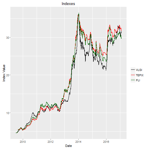
Ploting Value line geometric index with variable stocks, TEPIX, and FLOATING index, the last to are scaled to the value line range. We see some differences, and sharper reactions in case of value line.
Conclusion
Out-of-sample RMSE shows that my guesses are not rejected:
- Iliquid stocks affect index
- reported indexes are not best option for prediction
- Taking a variable set of stock as basis yield better results
In the next post I will see how clustering will affect the results.